Bernoulli Schemes with a finite alphabet
We are concerned with sequences of very long words \((x_0,x_1,x_2,\ldots)\), where each \(x_i\) is taken from a finite alphabet \(\mathcal A:=\{a,b,\ldots\}\). We will consider infinitely-long words, which is a standard approach if the words length is much larger than the number of iterations of the shift map (defined below). These structures are a basic building block for Statistical Mechanics, Dynamical Systems and Finite Automata. Here we investigate the simplest example, the case where we sample each letter independently.
This page contains interactive content, feel free to explore and modify it. For more involved modifications, you are encouraged to run and edit the interactive Jupyter Notebook instead. You can either:
- Run it on a computer with a Python/Jupyter-lab installation (requires
ipywidgets,numpy,matplotlib). - Run it using an online service. The official Jupyter website provides a free and open service. If you need more computing power, you can import the notebook in Google Colab (requires a Google account).
Definitions
Let \(\mathcal A\) be a finite or countable set and let \(M\colon \mathcal A\times \mathcal A\to \{0,1\}\). \(\mathcal A\) represents the alphabet, and \(M\) encodes which pairs of letters can be consecutive (more complex rules for the allowed sequences of letters fit within this framework just by modifying the alphabet space).
The space \(\Sigma \equiv \Sigma(\mathcal A,M)\) of \(M\)-compatible words is the space of sequences \[ \Sigma:= \left\{ x \in \mathcal A^{\mathbb N} \,:\: M_{x_i,x_{i+1}}=1,\,\forall i\in \mathbb N \right\} \] In other words, \(M\) tells us which letters can be consecutive, and \(\Sigma\) is the space of infinitely long words that only contain consecutive pairs of allowed letters. \(\Sigma\) is a measurable space, being a measurable subset of \(\mathcal A^{\mathbb N}\) (equipped with the product \(\sigma\)-algebra). Elements of \(\Sigma\) are usually denoted by \(x,y,z\), and we write \(x=(x_0,x_1\ldots)\) and so on.
Definition 1 (Shift map) The map \[ \begin{aligned} & T \colon \Sigma\to \Sigma \\ & (Tx)_i=x_{i+1} \end{aligned} \] is called the shift map.
Usually the pair \((\mathcal A, M)\) (and thus the ensuing space \(\Sigma\) equipped with the shift map \(T\)) is called a symbolic dynamical system.
Notice that \(T\) is not invertible (unless \(\mathcal A\) has just one element), since the first letter of \(x\) disappears in \(Tx\), the second letter becomes the first, and so on.
Definition 2 (Invariant measure) A probability measure \(\mathbb P\) on \(\Sigma\) is called invariant if \[ \begin{aligned} \mathbb P( E)=\mathbb P(T^{-1}(E)) \end{aligned} \tag{1}\]
Let \(\mu \in \mathcal P(\mathcal A)\) be a probability measure on \(\mathcal A\). If \(M_{a,b}=1\) for all \(a,b\in \mathcal A\), then the product measure \(\mathbb P= \mu^{\otimes \mathbb N}\) is invariant. This statement is obvious, it is just a difficult way of saying that \[ \mathbb P(X_{0}\in A_0,\ldots, X_{n-1} \in A_{n-1})= \mathbb P(X_{1}\in A_0,\ldots, X_{n} \in A_{n-1}) \] if the \(X_i\) are i.i.d.. Indeed, by the definition of the product \(\sigma\)-algebra, it is enough to check Equation 1 for cylindrical sets \(E=A_0\times \cdots A_{n-1} \times \mathcal A \times \dots \mathcal A\).
Definition 3 (Bernoulli Scheme) A Bernoulli Scheme is a symbolic dynamical system where \(\mathcal A\) is finite or countable, \(M_{a,b}=1\) for all \(a,b \in \mathcal A\), and \(\mathbb P=\mu^{\otimes \mathbb N}\) is a product probability measure on \(\Sigma=\mathcal A^{\mathbb N}\), for some probability \(\mu\) on \(\mathcal A\). In other words, it is just a sequence of i.i.d. random variables over a finite or countable space \(\mathcal A\), each with distribution \(\mu\). If \(\mathcal A\) is finite, then the scheme is called finite.
Example 1 Consider a Bernoulli scheme over the alphabet \(\mathcal A=\{0,1\}\). This is identified by a parameter \(p\in [0,1]\) given by \(p=\mu(\{1\})\). To avoid trivial situations, we choose \(p\in (0,1)\). Up to a countable set (and thus a set of \(\mathbb P\)-measure \(0\)), \(\Sigma=\{0,1\}^{\mathbb N}\) is in bijection with the interval \([0,1]\) via the map \[ \Phi(x):= \sum_{i\ge 0} 2^{-i-1} x_i \] The point \(\Phi(x)\) will be in the interval \([0,1/2)\) if \(x_0=0\), and in the interval \([1/2,1]\) if \(x_0=1\). Similarly \(\Phi(x)\in [0,1/4)\) if \(x_0=0\) and \(x_1=0\), \(\Phi(x)\in [1/4,1/2)\) if \(x_0=0\) and \(x_1=1\), and so on. This is not entirely exact, since dyadic numbers admit two binary representations, e.g. \(\Phi(01111111\ldots)=1/2=\Phi(10000000\ldots)\). But this is just a countable set that we will neglect since it has measure \(0\) (it is possible to make \(\Phi\) bijective and measurable changing its definition on a countable set but we do not need it here).
So we can look at this Bernoulli scheme on \([0,1]\) instead. What does the shift map \(x\mapsto Tx\) correpond to? In other words, can we identify a map \(T'\colon [0,1]\to [0,1]\) such that \(T'(\Phi(x))=\Phi(Tx)\)? This is just a way of saying: I first change the space to represent my points, from \(\Sigma \ni x\) to \([0,1] \ni \Phi(x)\). Now \(x\) changes to \(Tx\), can I read this change autonomously on \([0,1]\), just a function of the image \(\Phi(x)\)? Of course we can, since \(\Phi\) is invertible a.e.. So \(T'y=\Phi( T \Phi^{-1}y)\). We claim that \(T'y= 2y (\mathrm{mod} 1)\); which it is easy to check. Indeed \[ \Phi(Tx)= \sum_{i\ge 0} 2^{-i-1}x_{i+1}= \begin{cases} 2\Phi(x) & \text{if $x_0=0$} \\ 2\Phi(x) -1 & \text{if $x_0=1$} \end{cases} \]
Finite Schemes
Let us focus on finite Bernoulli schemes. So let \(\mathcal A=\{0,1,\ldots,n-1\}\), \(\Sigma=\mathcal A^{\mathbb N}\) and \(p_k:=\mu(\{k\})\) so that \(\sum_i p_i=1\). We assume \(p_i>0\) (otherwise just neglect the letters of the alphabet with \(0\) probability). As in Example 1 consider the \(n\)-ary representation \[ \begin{aligned} & \Phi \colon \Sigma \to [0,1] \\ & \Phi(x):= \sum_{i\ge 0} n^{-i-1} x_i \end{aligned} \]
Exercise 1 Prove that in this case, the \(n\)-ary representation pushes the shift map on \(\Sigma\) to the map \([0,1]\ni y \mapsto n y (\mathrm{mod} 1)\) on \([0,1]\).
We want to answer the following question. Fix \(\mu\), that is fix \(p_0, \ldots, p_{n-1}\). What is the pushforward of the measure \(\mathbb P=\mu^{\otimes \mathbb N}\) to \([0,1]\). In other words, if we take \((X_i)_{i \ge 0}\) i.i.d. with distribution \(\mu\) (so \(\mathbb P(X_i=k)=p_k\)) what will be the distribution of the random variable \[ Y= \sum_{i\ge 0} n^{-i-1} X_i \] The sum on the r.h.s. is well-defined, so \(Y\) is well-defined and we want to investigate its distribution. Let us denote \(\mathbb Q_{\mu}= \mu^{\otimes \mathbb N} \circ \Phi^{-1}\) the law of \(Y\) when the \(X_i\) are i.i.d. with distribution \(\mu\).
Proposition 1 If \(p_k\equiv p=1/n\), namely if the \(X_i\) are uniformly on the finite set \(\mathcal A\), then \(\mathbb Q_\mu\) is the Lebesgue measure (but defined on the Borel \(\sigma\)-algebra) on \([0,1]\).
Proof (Proposition 1). Indeed, we fix an interval of type \(I= [kn^{-j},(k+1)n^{-j}]\), for some \(j\ge 1\) and \(0\le k\le n^{j}-1\). We will have that \(Y=\Phi(X)\in I\) iff \(\sum_{i=0}^{j-1} n^{-i-1}X_i=kn^{-j}\) (up to a countable set of measure \(0\)). In turn, this holds for a unique value of \((X_0,\ldots,X_{j-1})\). Therefore \[ \mathbb Q_\mu(I)= \mathbb P(Y\in I)= \mathbb P\left(\sum_{i=0}^{j-1} n^{-i-1}X_i=kn^{-j}\right)= p^{j}= n^{-j}=\mathrm{Leb}(I) \] Since intervals of this type determine the measure entirely, we have \(\mathbb Q_\mu=\mathrm{Leb}\).
In other words, we can just obtain the Lebesgue measure by flipping a coin countably many times, a rather intuitive construction for an object that was ill-defined until the beginning of the 20th century. By the law of large numbers, Proposition 1 means that Lebesuge-almost all real numbers have the same frequency of each digit. Say, if we fix \(n=10\), then define \(\eta_{k,\ell}(x)\) the number of times a digit \(k=0,1,2,3,4,5,6,7,8,9\) occurs in the representation of \(x\) in base \(10\), in the first \(\ell\) digits of \(x\). Then \[ \mathrm{Leb}\left(\left\{x\in [0,1] \,:\: \limsup_\ell \frac{\eta_{k,\ell}}{\ell} =\liminf_\ell \frac{\eta_{k,\ell}}{\ell} = \frac{1}{10} \right\} \right)=1 \] Indeed, once we are back to the \(n=10\)-ary representation, \(\eta_{k,\ell}\) is nothing but the sum \(\sum_{i=0}^{\ell-1} \mathbf{1}_{X_i=k}\), which is a sum of i.i.d. random variables with expected value \(1/n\). So the strong law of large numbers implies that the limit exists and equals \(1/10\) with probability \(1\).
Theorem 1 For a probability \(\mu\in \mathcal P(\mathcal A)\), \(\mu(\{k\}):=p_k\) over the finite alphabet \(\mathcal A=\{0,\ldots,n-1\}\), define \[ E_\mu:= \left\{x\in [0,1] \,:\: \limsup_\ell \frac{\eta_{k,\ell}}{\ell}= \liminf_\ell \frac{\eta_{k,\ell}}{\ell}= p_k, \quad \forall k \in \mathcal A \right\} \] Then the \(E_\mu\) are measurable, disjoint sets and \(\mathbb Q_\mu(E_\mu)=1\) (and thus \(\mathbb Q_\mu(E_{\mu'})=0\) for \(\mu \neq \mu'\)). Thus
- If \(\mu\) is uniform, namely if \(p_k=1/n\), \(\mathbb Q_\mu\) is the Lebesgue measure.
- If there exists \(k\in \mathcal A\) such that \(p_k=1\), then \(\mathbb Q_\mu\) is Dirac mass (it is concentrated on one point).
- If \(p_k<1\) for all \(k\), but the measure is not uniform, \(\mathbb Q_\mu\) is of Cantor type, namely it gives measure \(0\) to every point, but is singular w.r.t. the Lebesgue measure.
The proof is left as a guided exercise.
Exercise 2
- Notice that, by their very definition, the \(E_\mu\) are Borel-measurable and disjoint.
- Reasoning as in the text after Proposition 1, prove in detail that \(\mathbb Q_\mu(E_\mu)=1\).
- Recall Proposition 1 and solve the trivial case where \(p_k=1\) for some \(k\), to prove the statements A) and B) in the theorem.
- In the case C), it remains to prove that \(\mathbb Q_\mu\) gives measure \(0\) to each point.
Testing convergence
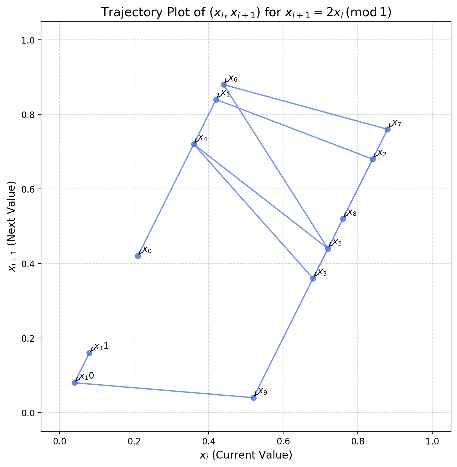
We can look at the trajectory of points of the map \(x\mapsto nx (\pmod 1)\).
#| '!! shinylive warning !!': |
#| shinylive does not work in self-contained HTML documents.
#| Please set `embed-resources: false` in your metadata.
#| standalone: true
#| components: [editor, viewer]
#| viewerHeight: 1080
#| editorHeight: 240
#| layout: vertical
from shiny import App, render, ui, reactive, req
import numpy as np
import matplotlib.pyplot as plt
# ========= 1. UI DEFINITION =========
# The UI remains exactly the same.
app_ui = ui.page_sidebar(
ui.sidebar(
ui.h4("Iteration Graph"),
ui.input_slider("n", "Multiplier (n):", min=2, max=10, value=2, step=1),
ui.input_slider("iterations", "Number of Steps:", min=1, max=20, value=10, step=1),
ui.input_slider("x0", "Initial Value (x0):", min=0.0, max=1.0, value=0.21, step=0.01),
ui.input_action_button("generate_button", "Generate Graph", class_="btn-success"),
ui.hr(),
ui.input_checkbox("save_plot", "Save Plot", value=False),
ui.panel_conditional(
"input.save_plot",
ui.input_text("filename", "Filename:", value="graph.png"),
),
title="Controls",
),
ui.output_plot("map_plot", height="600px"),
title="Plot of pairs (x_{i},x_{i+1})",
)
# ========= 2. SERVER LOGIC =========
def server(input, output, session):
# This reactive.Value still acts as the bridge between the action and the render output.
figure_to_display = reactive.Value(None)
def generate_map_sequence(n, num_iterations, x0):
"""Generates a sequence using the map x_{i+1} = n*x_i (mod 1)."""
seq = np.zeros(num_iterations + 1)
seq[0] = x0
for i in range(num_iterations):
seq[i+1] = (n * seq[i]) % 1.0
return seq
# This is the corrected way to perform an action when a button is clicked.
# @reactive.event specifies the trigger.
# @reactive.Effect specifies that this function performs a side-effect.
@reactive.Effect
@reactive.event(input.generate_button, ignore_init=True)
def _():
"""This function runs ONLY when the generate_button is clicked."""
n = input.n()
num_iterations = input.iterations()
x0 = input.x0()
try:
sequence = generate_map_sequence(n, num_iterations, x0)
x_points = sequence[:-1]
y_points = sequence[1:]
fig, ax = plt.subplots(figsize=(8.5, 8.5))
ax.plot(x_points, y_points, 'o-', color='royalblue', markersize=6, alpha=0.7)
for i in range(num_iterations):
ax.annotate(f'$x_{i}$',
xy=(x_points[i], y_points[i]),
xytext=(5, 5),
textcoords='offset points')
ax.set_title(f'Trajectory Plot of $(x_i, x_{{i+1}})$ for $x_{{i+1}} = {n} x_i \\, (\\mathrm{{mod}}\\,1)$', fontsize=12)
ax.set_xlabel('$x_i$ (Current Value)', fontsize=12)
ax.set_ylabel('$x_{i+1}$ (Next Value)', fontsize=12)
ax.set_xlim(-0.05, 1.05)
ax.set_ylim(-0.05, 1.05)
ax.set_aspect('equal', adjustable='box')
ax.grid(True, linestyle='--', alpha=0.5)
if input.save_plot():
req(input.filename(), cancel_output=True)
fig.savefig(input.filename(), dpi=400)
# Set the reactive value, which will cause the plot output to update.
figure_to_display.set(fig)
except Exception as e:
fig, ax = plt.subplots()
ax.text(0.5, 0.5, f"An error occurred: {e}", ha='center', va='center')
figure_to_display.set(fig)
@output
@render.plot
def map_plot():
# This render function simply displays the figure held in our reactive.Value.
fig = figure_to_display.get()
# Don't render an empty output before the button is first clicked.
req(fig)
return fig
# ========= 3. APP INSTANTIATION =========
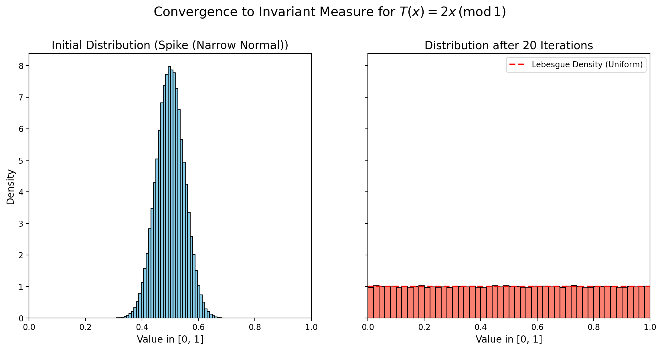
app = App(app_ui, server)We can check that if we start with \(N\) points sampled with a given distribution \(\mu\), we can see numerically that in a few step they will spread out along the interval. The idea is that, if we start with a distribution \(\mu\) absolutely continuous w.r.t. an invariant measure, then after many iterations of the shift map \(T\), the distribution of points will get close to the invariant measure (Lebesgue).
However, Lebesgue is not the only invariant measure, and as we iterate the map many times, we see the problems. Numerical precision (the fact that we cannot exactly sample a.c. w.r.t. Lebesgue) will have an impact when we iterate the map many times, e.g. periodic orbits (that have \(0\) probability w.r.t. Lebesgue) have positive probability when we sample on a computer. The effect is visible in this video.
Feel free to experiment how different distributions converge to Lebesgue. Can you imagine how to mathematically state a convergence result?
#| '!! shinylive warning !!': |
#|   shinylive does not work in self-contained HTML documents.
#|   Please set `embed-resources: false` in your metadata.
#| standalone: true
#| components: [editor, viewer]
#| viewerHeight: 1080
#| editorHeight: 240
#| layout: vertical

from shiny import App, render, ui, reactive, req
import numpy as np
import matplotlib.pyplot as plt

# ========= 1. UI DEFINITION =========
# The UI is structured with controls in a sidebar and the main plot output.
# The descriptive text below the plot has been removed as requested.
app_ui = ui.page_sidebar(
    ui.sidebar(
        ui.h4("Simulation Controls"),
        ui.input_slider("n_slider", "Multiplier (n):", min=2, max=10, value=2, step=1),
        ui.input_slider("num_points_slider", "Number of Points:", min=10000, max=500000, value=100000, step=10000),
        ui.input_slider("num_iterations_slider", "Number of Iterations:", min=1, max=50, value=20, step=1),
        ui.input_select("distribution", "Initial Distribution:",
                        choices=['Spike (Narrow Normal)', 'Uniform (Lebesgue)', 'Periodic Points'],
                        selected='Spike (Narrow Normal)'),
        ui.input_action_button("run_button", "Run Simulation", class_="btn-success"),
        ui.hr(),
        ui.h4("Plotting & Saving"),
        ui.input_checkbox("save_plot", "Save Plot", value=False),
        ui.panel_conditional(
            "input.save_plot",
            ui.input_text("filename", "Filename:", value="measure_invariance.png"),
        ),
        title="Controls",
    ),
    ui.output_plot("measure_plot", height="600px"),
    title="Convergence to invariant measures",
)

# ========= 2. SERVER LOGIC =========
def server(input, output, session):
    figure_to_display = reactive.Value(None)

    def generate_and_iterate(dist_name, num_points, n, num_iterations):
        """Generates initial points and iterates the map on all of them."""
        if dist_name == 'Uniform (Lebesgue)':
            initial_points = np.random.rand(num_points)
        elif dist_name == 'Spike (Narrow Normal)':
            initial_points = np.mod(np.random.normal(loc=0.5, scale=0.05, size=num_points), 1.0)
        elif dist_name == 'Periodic Points':
            # Points are concentrated around rational periodic orbits, which converge slowly.
            if n == 2:
                # For n=2, the orbit {1/3, 2/3} is a classic period-2 orbit.
                base_points = [1/3, 2/3]
            else:
                # For n>2, points k/(n-1) are fixed points (period 1).
                base_points = [1/(n-1), 2/(n-1)]

            num_bases = len(base_points)
            points_per_base = num_points // num_bases

            all_samples = []
            for i, base in enumerate(base_points):
                # Distribute points evenly among bases, giving remainder to the last one.
                current_num_points = points_per_base if i < num_bases - 1 else num_points - (points_per_base * (num_bases - 1))
                # Create a very narrow spike around the periodic point.
                samples = np.random.normal(loc=base, scale=1e-6, size=current_num_points)
                all_samples.append(samples)

            initial_points = np.mod(np.concatenate(all_samples), 1.0)
            np.random.shuffle(initial_points)
        else:
            raise ValueError(f"Unknown distribution: {dist_name}")

        final_points = initial_points.copy()
        for _ in range(num_iterations):
            final_points = (n * final_points) % 1.0

        return initial_points, final_points

    @reactive.Effect
    @reactive.event(input.run_button, ignore_init=True)
    def _():
        """This function runs when the 'Run Simulation' button is clicked."""
        n = input.n_slider()
        num_points = input.num_points_slider()
        num_iterations = input.num_iterations_slider()
        dist_name = input.distribution()

        try:
            initial, final = generate_and_iterate(dist_name, num_points, n, num_iterations)

            fig, (ax1, ax2) = plt.subplots(1, 2, figsize=(14, 6), sharey=True)

            ax1.hist(initial, bins=50, density=True, color='skyblue', edgecolor='black')
            ax1.set_title(f'Initial Distribution ({dist_name})', fontsize=14)
            ax1.set_xlabel('Value in [0, 1]', fontsize=12)
            ax1.set_ylabel('Density', fontsize=12)
            ax1.set_xlim(0, 1)
            ax1.grid(True, linestyle='--', alpha=0.5)

            ax2.hist(final, bins=50, density=True, color='salmon', edgecolor='black')
            ax2.set_title(f'Distribution after {num_iterations} Iterations', fontsize=14)
            ax2.set_xlabel('Value in [0, 1]', fontsize=12)
            ax2.set_xlim(0, 1)
            ax2.axhline(1.0, color='red', linestyle='--', linewidth=2, label='Lebesgue Density (Uniform)')
            ax2.legend()
            ax2.grid(True, linestyle='--', alpha=0.5)

            # fig.suptitle(f'Convergence to Invariant Measure for $T(x) = {n}x \\, (\\mathrm{{mod}}\\,1)$', fontsize=16, y=1.02)

            if input.save_plot():
                req(input.filename(), cancel_output=True)
                fig.savefig(input.filename(), dpi=400, bbox_inches='tight')

            figure_to_display.set(fig)

        except Exception as e:
            fig, ax = plt.subplots()
            ax.text(0.5, 0.5, f"An error occurred: {e}", ha='center', va='center', color='red')
            figure_to_display.set(fig)

    @output
    @render.plot
    def measure_plot():
        """Renders the plot held in the reactive value."""
        fig = figure_to_display.get()
        req(fig)
        return fig

# ========= 3. APP INSTANTIATION =========
app = App(app_ui, server)