Central Limit Theorem
This is a quick review of the Central Limit Theorem (CLT), trying to give a concrete meaning to the nature of the convergence (in distribution, not in probability).
This page contains (at its end) interactive content, feel free to explore and modify it. For more involved modifications, you are encouraged to run and edit the interactive Jupyter Notebook instead. You can either:
- Run it on a computer with a Python/Jupyter-lab installation (requires
ipywidgets,numpy,matplotlib). - Run it using an online service. The official Jupyter website provides a free and open service. If you need more computing power, you can import the notebook in Google Colab (requires a Google account).
Convergence Results
Let us review some basic convergence results for sums of centered random variables with finite variance.
The classical statement
Theorem 1 (Central Limit Theorem) Let \((X_n)_{n\ge 1}\) be an i.i.d. sequence of real-valued random variables with \(\mathbb E[|X_n|^2]<\infty\). Denote \(m:= \mathbb E[X_n]\), \(\sigma:= \sqrt{\mathrm{Var}[X_n]}\) and \[ S_n:= \frac{1}{\sqrt{n}} \sum_{i=1}^n \frac{X_i -m}{\sigma} \tag{1}\] Then \(S_n\) converges in distribution to a standard normal random variable, say \(Z\sim \mathcal N(0,1)\). In other words, for each bounded measurable function \(f \colon \mathbb R\to \mathbb R\) which is continuous a.e., it holds \[ \lim_{n\to \infty} \mathbb E[f(S_n)] = \frac{1}{\sqrt{2 \pi}} \int f(x) e^{-x^2/2} dx \]
In particular one can deduce uniform convergence of the distribution function from the previous theorem \[ \lim_{n\to \infty} \sup_{a<b}\left| \mathbb P( a< S_n \le b) - \mathbb P(a<Z\le b)\right|=0 \]
A quantitative version
The previous Theorem 1 does not address the rate of convergence.
Theorem 2 (Quantitative Central Limit Theorem) Let \((Y_n)_{n\ge 1}\) be a sequence of independent random variables with \(\mathbb E[Y_n]=0\) and \(\mathbb E[Y_n^2]=1\), \(\mathbb E[|Y_n|^3]<\infty\). Let \[ S_n:= \frac{1}{\sqrt{n}} \sum_{i=1}^n Y_i \] For \(g\in C^3_b(\mathbb R)\) with \(C:= \sup_x |g'''(x)|\), the following inequality holds \[ |\mathbb E[g(S_n)] - \mathbb E[g(Z)]| \le \frac{C}{6\sqrt{n}} \left( \frac{2^{3/2}}{\sqrt{\pi}}+\frac{1}{n}\sum_{k=1}^n \mathbb E[|Y_k|^3] \right) \] where \(Z\sim \mathcal N(0,1)\); namely \[ \mathbb E[g(Z)] = \tfrac{1}{\sqrt{2 \pi}} \int g(x) e^{-x^2/2} dx \]
Lemma 1 Let \(V\), \(Y\), and \(Z\) be three random variables, such that
- \(V\) and \(Y\) are independent; \(V\) and \(Z\) are independent.
- \(Y\) and \(Z\) have a finite third moment.
- \(\mathbb E[Y] = \mathbb E[Z]\) and \(\mathbb E[Y^2] =\mathbb E[Z^2]\).
Then for any \(g \in C_b^3\), setting \(C := \sup_{x \in \mathbb{R}} |g'''(x)|\), the following inequality holds: \[ |\mathbb E[g(V +Y )] - \mathbb E[g(V + Z)]| \le \frac{C}{6} \left( \mathbb E[|Y|^3] + \mathbb E[|Z|^3] \right) \]
Proof (Lemma 1). By Taylor expansion, for three points \(v,y,z \in \mathbb R\) it holds \[ g(v+y)-g(v+z)= g'(v) (y-z) + \tfrac 12 g''(v)(y^2-z^2) + R(v,y)- R(v,z) \] where the remainder terms \(R(v,\cdot)\) are bounded as \(|R(v,x)|\le C |x|^3/6\). Computing the last formula at \(v=V(\omega)\), \(y=Y(\omega)\) and \(z=Z(\omega)\), then taking expectation, one gathers \[ \left| \mathbb E[g(V+Y)-g(V+Z)] \right| = \left| \mathbb E[R(V,Y) - R(V,Z)] \right| \le \frac{C}{6} \left( \mathbb E[|Y|^3] + \mathbb E[|Z|^3] \right) \] since (using the independence and equal expectation hypotheses) \(\mathbb E[g'(V) (Y-Z)]=\mathbb E[g'(V)] \mathbb E[(Y-Z)]=0\), and reasoning similarly \(\mathbb{E}[g''(V)(Y^2-Z^2)]=0\).
Lemma 2 Let \(g \in C^3_b(\mathbb R)\), let \(Y_1,\ldots,Y_n\) be independent random variables, and \(Z_1,\ldots,Z_n\) be another set of independent random variables. Assume \(\mathbb E[Y_i]=\mathbb E[Z_i]\), and \(\mathbb E[Y_i^2]= \mathbb E[Z_i^2]<\infty\). Let \(C\) be as in Lemma 1. Then \[ \left|\mathbb E\left[g\left(\tfrac{Y_1+\ldots+Y_n}{\sqrt{n}}\right) - g\left(\tfrac{Z_1+\ldots+Z_n}{\sqrt{n}}\right) \right] \right| \le \frac{C}{6 n^{3/2}}\sum_{k=1}^{n} \left( \mathbb E[|Y_k|^3] + \mathbb E[|Z_k|^3]\right) \] In particular if the \(Y_i\) are i.i.d. and the \(Z_i\) are i.i.d. (in general with a different distribution) \[ \left|\mathbb E\left[g\left(\tfrac{Y_1+\ldots+Y_n}{\sqrt{n}}\right) - g\left(\tfrac{Z_1+\ldots+Z_n}{\sqrt{n}}\right) \right] \right| \le \frac{C \left( \mathbb E[|Y_1|^3] + \mathbb E[|Z_1|^3] \right)}{6 \sqrt{n}} \]
Proof (Lemma 2). With no loss of generality, one can assume that all the \(Y_1,\ldots,Y_n,Z_1,\ldots,Z_n\) are independent random variables. Then write \(V_k=(Y_1+\ldots +Y_{k-1} + Z_{k+1}+\ldots +Z_{n})/\sqrt{n}\) to get \[ \begin{aligned} \left| \mathbb E\left[g\left(\tfrac{Y_1+\ldots+Y_n}{\sqrt{n}}\right) - g\left(\tfrac{Z_1+\ldots+Z_n}{\sqrt{n}}\right) \right] \right| & = \left| \sum_{k=1}^{n} \mathbb E\left[g\left(V_k + \tfrac{Y_{k}}{\sqrt{n}}\right) - g\left(V_k+\tfrac{Z_{k}}{\sqrt{n}}\right) \right] \right| \\ & \le \sum_{k=1}^{n} \frac{C}6 \left( \mathbb E[|Y_k/\sqrt{n}|^3] + \mathbb E[|Z_k/\sqrt{n}|^3]\right) \end{aligned} \] where in the last inequality we used Lemma 1 \(n\) times.
Proof (Theorem 2). If the \(Z_i\) are i.i.d. standard normal, then \((Z_1+\ldots + Z_n)/\sqrt{n}\) is also a standard normal and thus its distribution does not depend on \(n\). Theorem 2 is therefore a consequence of Lemma 2 and the identity \(\mathbb E[|Z_i|^3]=2^{3/2}/\sqrt{\pi}\).
Exercise 1 Let \(Z\sim \mathcal N(0,1)\) be a standard normal random variable. Let \((Y_n)_{n\ge 1}\) be an i.i.d. sequence with \(\mathbb E[Y_i^k]= \mathbb E[Z^k]\) for \(k=1,\ldots, \ell\). Let \(g\in C^\ell_b(\mathbb R)\). Prove that there exists a constant \(C\) (depending on \(g\) and the distribution of the \(Y_i\)) such that \[ \left| \mathbb E[g(S_n)]-\mathbb E[g(Z)] \right| \le C n^{-(\ell-1)/2} \]
A martingale version
It is worth mentioning that the Central Limit Theorem extends far beyond the scope of independent random variables.Ultimately, this type of result does not even need the variables to be defined on a linear space (e.g. making small random steps on a manifold will, as the steps decrease, converge to a distribution over continuous curves on the manifold, called Brownian Motion). So there are strong local versions of the CLT, metric-space versions, ergodic versions, and so on. An interesting example that only requires elementary hypotheses covers the case of martingales.
Theorem 3 (Martingale Central Limit Theorem) Let \((X_n)_{n\ge 1}\) be a sequence of real-valued random variables and let \[ M_n:= X_1+\ldots+X_n \] Assume that
- \(\mathbb E[X_n| M_{n-1}]=0\).
- For \(Q_n:= \mathbb E[X_n^2| M_{n-1} ]\), it holds \(\sum_{n=1}^\infty Q_n=\infty\) a.s..
- \(\mathbb E\left[\sup_n \mathbb E[|X_n|^3| M_{n-1} ] \right]<\infty\).
Let \(\tau_\ell:=\inf \{N\in \mathbb N \,:\: \sum_{n=1}^N Q_n \ge \ell\}\). Then \(M_{\tau_\ell}/\sqrt{\ell}\) converges to a standard normal in distribution as \(\ell \to \infty\).
Non-Convergence Results
So far so good. If the \(Y_n\) are centered i.i.d. random variables with finite variance \(S_n\) converges to a normal limit. In distribution. Will this convergence hold in probability or even a.s.?
Proposition 1 Regardless of the probability space and the distribution of the \(Y_n\), the Central Limit Theorem does not hold in probability, not even along subsequences.
The point is that if two sequences \((S_n), (S_n')\) converge in probability, then \(S_n+S_n'\) converges in probability (by triangular inequality). The same statement does not hold in distribution, since convergence in distribution does not concern the random variables, but only their distribution. Thus the convergence of \(S_n\) or \(S_n'\) says nothing about their joint distribution.
Proof (Proposition 1). Any limit point (along some subsequence) in probability \(S\) of \(S_n\), will have a standard normal distribution. In particular \(\sqrt{2} S_{2n}-S_n\) would converge to \((\sqrt{2}-1) S \sim \mathcal N(0,3-2\sqrt{2})\) in probability (along the same subsequence). But \[ S_n':= \sqrt{2} S_{2n} - S_n = \frac{1}{\sqrt{n}}\sum_{i=n+1}^{2n} Y_i \] is a sum of \(n\) i.i.d. divided by \(\sqrt{n}\), thus the Theorem 1 applies to \(S'_n\). Namely for any limit point \(S\), \((\sqrt{2}-1) S\) should also have \(\mathcal{N}(0,1)\) law. Therefore there are no limit points.
Visualizing the Convergence
What does it mean that the sequence converges in distribution? Let’s fix \(\mu\), a centered probability measure on \(\mathbb R\), and some value \(n\) ‘large enough’ (as we have seen, how large depends on \(\mu\), for instance in its third moment) and let us consider i.i.d. \(X_1,\ldots,X_n\) with law \(\mu\) and the ensuing \(S_n\) as in Equation 1. We can sample many times, say \(N\), \((X_1,\ldots,X_n)\) and thus \(S_n\) independently. The Central Limit Theorem tells us that, with large probability, the fraction of samples for which \(S_n\) falls in a given interval \([a,b]\) is roughly equal to the gaussian integral over \([a,b]\). Here roughly means with a probability converging to \(1\) as \(N\) and \(n\) grow.
Here we take \(N\) samples, plot how many of them fall in each interval, and compare the result against the theoretical Gaussian density.
#| '!! shinylive warning !!': |
#|   shinylive does not work in self-contained HTML documents.
#|   Please set `embed-resources: false` in your metadata.
#| standalone: true
#| components: [editor, viewer]
#| viewerHeight: 1080
#| editorHeight: 240
#| layout: vertical

# ========= 1. IMPORTS & CONFIGURATION =========
from shiny import App, render, ui, reactive, req
import numpy as np
import matplotlib.pyplot as plt
from scipy.stats import norm, cauchy

# Configuration dictionary for UI inputs
DIST_CONFIG = {
    'n_slider': {
        'min': 10, 'max': 10000, 'value': 1000, 'step': 1,
    },
    'N_samples_slider': {
        'min': 100, 'max': 10000, 'value': 5000, 'step': 100,
    },
    'distribution': {
        'choices': ['{-1, +1} (Bernoulli)', 'Uniform [-1, 1]', 'Standard Normal N(0,1)', 'Centered Exponential (Exp(1)-1)', 'Standard Cauchy'],
        'selected': '{-1, +1} (Bernoulli)',
    },
    'filename': {'value': 'clt_distribution.png'},
}

# ========= 2. UI DEFINITION =========
app_ui = ui.page_sidebar(
    ui.sidebar(
        ui.h4("Convergence in Distribution"),
        ui.input_slider("n", "Sequence Length (n):", **DIST_CONFIG['n_slider']),
        ui.input_slider("N_samples", "Number of Samples (N):", **DIST_CONFIG['N_samples_slider']),
        ui.input_select("distribution", "Distribution:", **DIST_CONFIG['distribution']),
        ui.hr(),
        ui.input_action_button("run_button", "Run Simulation", class_="btn-success w-100"),
        ui.hr(),
        ui.h4("Saving Options"),
        ui.input_checkbox("save_plot", "Save Plot", value=False),
        ui.panel_conditional(
            "input.save_plot",
            ui.input_text("filename", "Filename:", **DIST_CONFIG['filename']),
        ),
        title="Controls",
    ),
    ui.output_plot("dist_plot", height="700px"),
    title="Distribution of the Normalized Sum",
)

# ========= 3. SERVER LOGIC =========
def server(input, output, session):
    # Reactive value to hold the generated matplotlib figure
    figure_to_display = reactive.Value(None)

    # --- Helper Functions (from original script) ---
    def dist_generate_steps(dist_name, size):
        if dist_name == '{-1, +1} (Bernoulli)': return np.random.choice([-1, 1], size=size)
        if dist_name == 'Uniform [-1, 1]': return np.random.uniform(-1, 1, size=size)
        if dist_name == 'Standard Normal N(0,1)': return np.random.randn(*size)
        if dist_name == 'Centered Exponential (Exp(1)-1)': return np.random.standard_exponential(size=size) - 1
        if dist_name == 'Standard Cauchy': return np.random.standard_cauchy(size=size)
        raise ValueError(f"Unknown distribution: {dist_name}")

    def dist_get_limit_pdf(dist_name, n):
        if dist_name in ['{-1, +1} (Bernoulli)', 'Standard Normal N(0,1)', 'Centered Exponential (Exp(1)-1)']:
            return 'Normal(0, 1)', lambda x: norm.pdf(x, loc=0, scale=1)
        if dist_name == 'Uniform [-1, 1]':
            # The variance of U[-1,1] is (1 - (-1))^2 / 12 = 4/12 = 1/3
            return 'Normal(0, 1/√3)', lambda x: norm.pdf(x, loc=0, scale=np.sqrt(1/3))
        if dist_name == 'Standard Cauchy':
            # The normalized sum of Cauchy variables is still Cauchy.
            # S_n / n ~ Cauchy(0,1), so S_n / sqrt(n) is not standard.
            # Let's assume the user wants to see the stable distribution, which is just Cauchy.
            return 'Cauchy(0, 1)', lambda x: cauchy.pdf(x, loc=0, scale=1)

    @reactive.Effect
    @reactive.event(input.run_button, ignore_init=True)
    def _():
        """This function runs ONLY when the run_button is clicked."""
        n = input.n()
        N = input.N_samples()
        dist_name = input.distribution()

        try:
            # Generate the sample data
            X = dist_generate_steps(dist_name, size=(N, n))
            # For Cauchy, the stable sum is normalized by n, not sqrt(n)
            if dist_name == 'Standard Cauchy':
                S_n_samples = np.sum(X, axis=1) / n
            else:
                S_n_samples = np.sum(X, axis=1) / np.sqrt(n)

            # Create the plot
            fig, ax = plt.subplots(figsize=(10, 6))
            num_bins = min(150, max(20, N // 100))
            ax.hist(S_n_samples, bins=num_bins, density=True, alpha=0.75, label=f'Empirical Dist. of $S_n$ (N={N:,})')

            # Get and plot the theoretical PDF
            limit_name, limit_pdf = dist_get_limit_pdf(dist_name, n)
            x_min, x_max = ax.get_xlim()
            # For Cauchy, the range can be very wide, so we limit it for plotting
            if dist_name == 'Standard Cauchy':
                x_min, x_max = -10, 10
            x_axis = np.linspace(x_min, x_max, 400)
            ax.plot(x_axis, limit_pdf(x_axis), 'r-', lw=2, alpha=0.9, label=f'Theoretical PDF: {limit_name}')

            ax.set_title(f'Distribution of Normalized Sum for $X_i \\sim$ {dist_name}')
            ax.set_xlabel('Value of the Normalized Sum')
            ax.set_ylabel('Probability Density')
            ax.legend()
            ax.grid(True, linestyle='--', alpha=0.6)
            ax.set_xlim(x_min, x_max) # Enforce x-limits

            # Save if requested
            if input.save_plot():
                req(input.filename(), cancel_output=True)
                fig.savefig(input.filename(), dpi=400, bbox_inches='tight')

            # Update the reactive value to display the plot
            figure_to_display.set(fig)
            plt.close(fig)

        except Exception as e:
            fig, ax = plt.subplots()
            ax.text(0.5, 0.5, f"An error occurred: {e}", ha='center', va='center', wrap=True)
            figure_to_display.set(fig)
            plt.close(fig)

    @output
    @render.plot
    def dist_plot():
        """Renders the plot from the reactive value."""
        fig = figure_to_display.get()
        req(fig)  # Do not render until the button is clicked
        return fig

# ========= 4. APP INSTANTIATION =========
app = App(app_ui, server)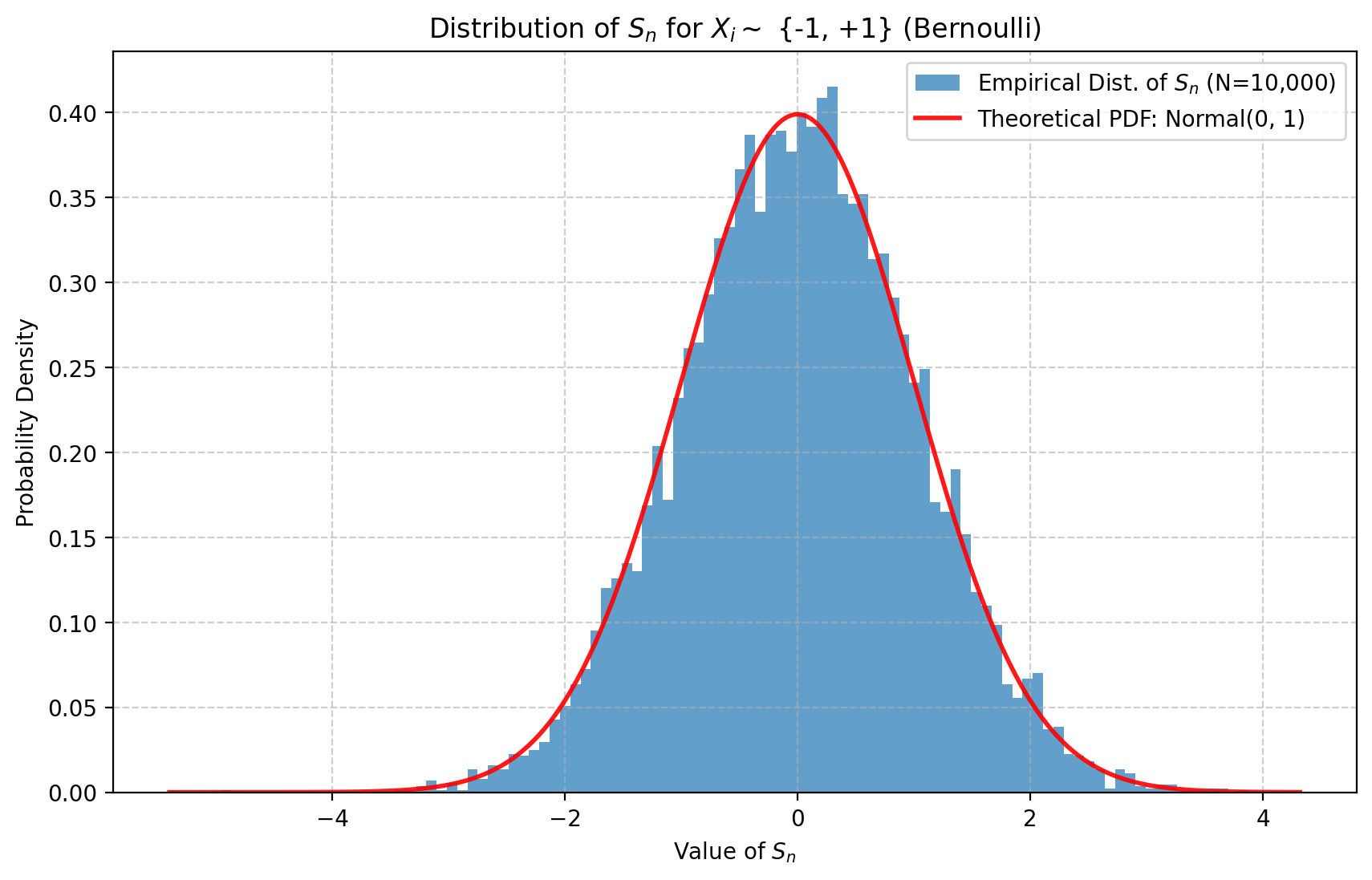
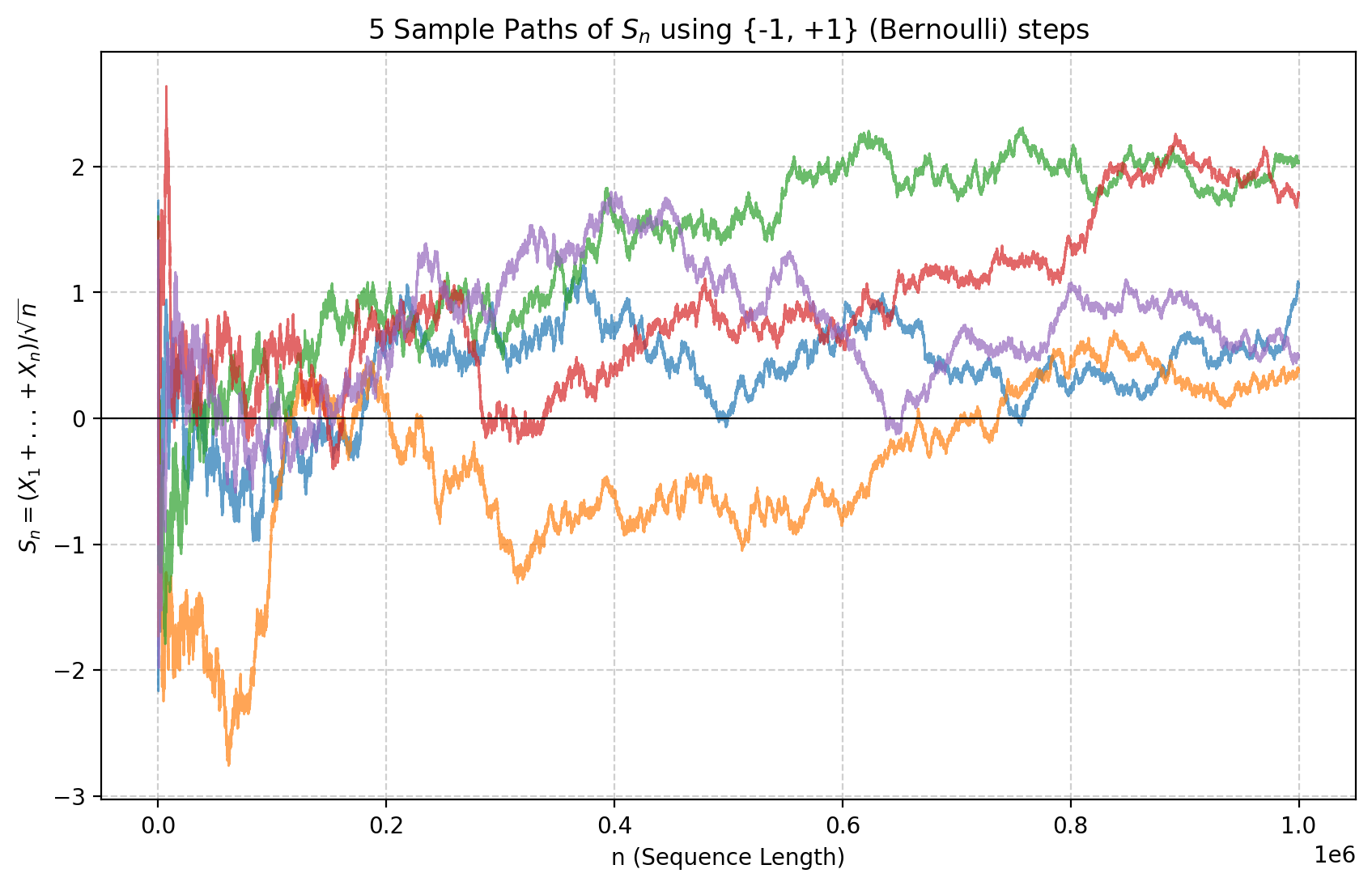
On the other hand, the fact that \(S_n\) is not converging a.s., means that if we fix a sample (an \(\omega\) so to speak) and we follow the value of \(S_n\) as depending on \(n\), it will not converge to any value.
Each individual sample does not converge as a function of \(n\): we extract the \(X_i\) i.i.d., and plot \(S_n\) as a function of \(n\). Even for \(n\) large, the plot oscillates and convergence does not set in.
#| '!! shinylive warning !!': |
#|   shinylive does not work in self-contained HTML documents.
#|   Please set `embed-resources: false` in your metadata.
#| standalone: true
#| components: [editor, viewer]
#| viewerHeight: 1080
#| editorHeight: 240
#| layout: vertical

# ========= 1. IMPORTS & CONFIGURATION =========
from shiny import App, render, ui, reactive, req
import numpy as np
import matplotlib.pyplot as plt

# Configuration dictionary for UI inputs
PATHS_CONFIG = {
    'n_slider': {
        'min': 1000, 'max': 1000000, 'value': 10000, 'step': 1000,
    },
    'N_slider': {
        'min': 1, 'max': 50, 'value': 5, 'step': 1,
    },
    'distribution': {
        'choices': ['{-1, +1} (Bernoulli)', 'Uniform [-1, 1]', 'Standard Normal N(0,1)', 'Standard Cauchy', 'Centered Exponential (Exp(1)-1)'],
        'selected': 'Standard Normal N(0,1)',
    },
    'linewidth_slider': {
        'min': 0.1, 'max': 3.0, 'value': 1.0, 'step': 0.1,
    },
    'filename': {'value': 'clt_paths.png'},
}

# ========= 2. UI DEFINITION =========
app_ui = ui.page_sidebar(
    ui.sidebar(
        ui.h4("Path Trajectory Simulation"),
        ui.input_slider("n", "Sequence Length (n):", **PATHS_CONFIG['n_slider']),
        ui.input_slider("N", "Number of Paths:", **PATHS_CONFIG['N_slider']),
        ui.input_select("distribution", "Distribution:", **PATHS_CONFIG['distribution']),
        ui.hr(),
        ui.h4("Plotting & Saving Options"),
        ui.input_slider("linewidth", "Line Width:", **PATHS_CONFIG['linewidth_slider']),
        ui.input_action_button("resample_button", "Resample & Plot", class_="btn-success w-100"),
        ui.hr(),
        ui.input_checkbox("save_plot", "Save Plot", value=False),
        ui.panel_conditional(
            "input.save_plot",
            ui.input_text("filename", "Filename:", **PATHS_CONFIG['filename']),
        ),
        title="Controls",
    ),
    ui.output_plot("paths_plot", height="600px"),
    title="CLT Paths",
)

# ========= 3. SERVER LOGIC =========
def server(input, output, session):
    # Reactive value to hold the generated matplotlib figure
    figure_to_display = reactive.Value(None)

    def paths_generate_steps(dist_name, size):
        """Generates random steps based on the selected distribution."""
        if dist_name == '{-1, +1} (Bernoulli)':
            return np.random.choice([-1, 1], size=size)
        if dist_name == 'Uniform [-1, 1]':
            return np.random.uniform(-1, 1, size=size)
        if dist_name == 'Standard Normal N(0,1)':
            return np.random.randn(*size)
        if dist_name == 'Standard Cauchy':
            return np.random.standard_cauchy(size=size)
        if dist_name == 'Centered Exponential (Exp(1)-1)':
            return np.random.standard_exponential(size=size) - 1
        raise ValueError(f"Unknown distribution: {dist_name}")

    @reactive.Effect
    @reactive.event(input.resample_button, ignore_init=True)
    def _():
        """This function runs ONLY when the resample_button is clicked."""
        dist_name = input.distribution()
        max_n = input.n()
        N_trajectories = input.N()
        line_width = input.linewidth()

        try:
            # Generate data
            X = paths_generate_steps(dist_name, size=(N_trajectories, max_n))
            cumulative_sums = np.cumsum(X, axis=1)
            n_axis = np.arange(1, max_n + 1)
            S_n = cumulative_sums / np.sqrt(n_axis)

            # Create plot
            fig, ax = plt.subplots(figsize=(10, 6))
            for i in range(N_trajectories):
                ax.plot(n_axis, S_n[i, :], alpha=0.7, linewidth=line_width)

            ax.set_title(f'{N_trajectories} Sample Paths of $S_n$ using {dist_name} steps')
            ax.set_xlabel('n (Sequence Length)')
            ax.set_ylabel('$S_n = (X_1 + ... + X_n) / \\sqrt{n}$')
            ax.grid(True, linestyle='--', alpha=0.6)
            ax.axhline(0, color='black', linewidth=0.8)

            # Save the plot if requested
            if input.save_plot():
                req(input.filename(), cancel_output=True)
                fig.savefig(input.filename(), dpi=400, bbox_inches='tight')

            # Set the reactive value, which will trigger the plot output to update
            figure_to_display.set(fig)

            # Close the figure object to free memory
            plt.close(fig)

        except Exception as e:
            # On error, create a plot showing the error message
            fig, ax = plt.subplots()
            ax.text(0.5, 0.5, f"An error occurred: {e}", ha='center', va='center', wrap=True)
            figure_to_display.set(fig)
            plt.close(fig)

    @output
    @render.plot
    def paths_plot():
        """Renders the plot held in the reactive value."""
        fig = figure_to_display.get()
        # Don't render anything until the button has been clicked at least once
        req(fig)
        return fig

# ========= 4. APP INSTANTIATION =========
app = App(app_ui, server)