Statistical properties of 1-d Random walks
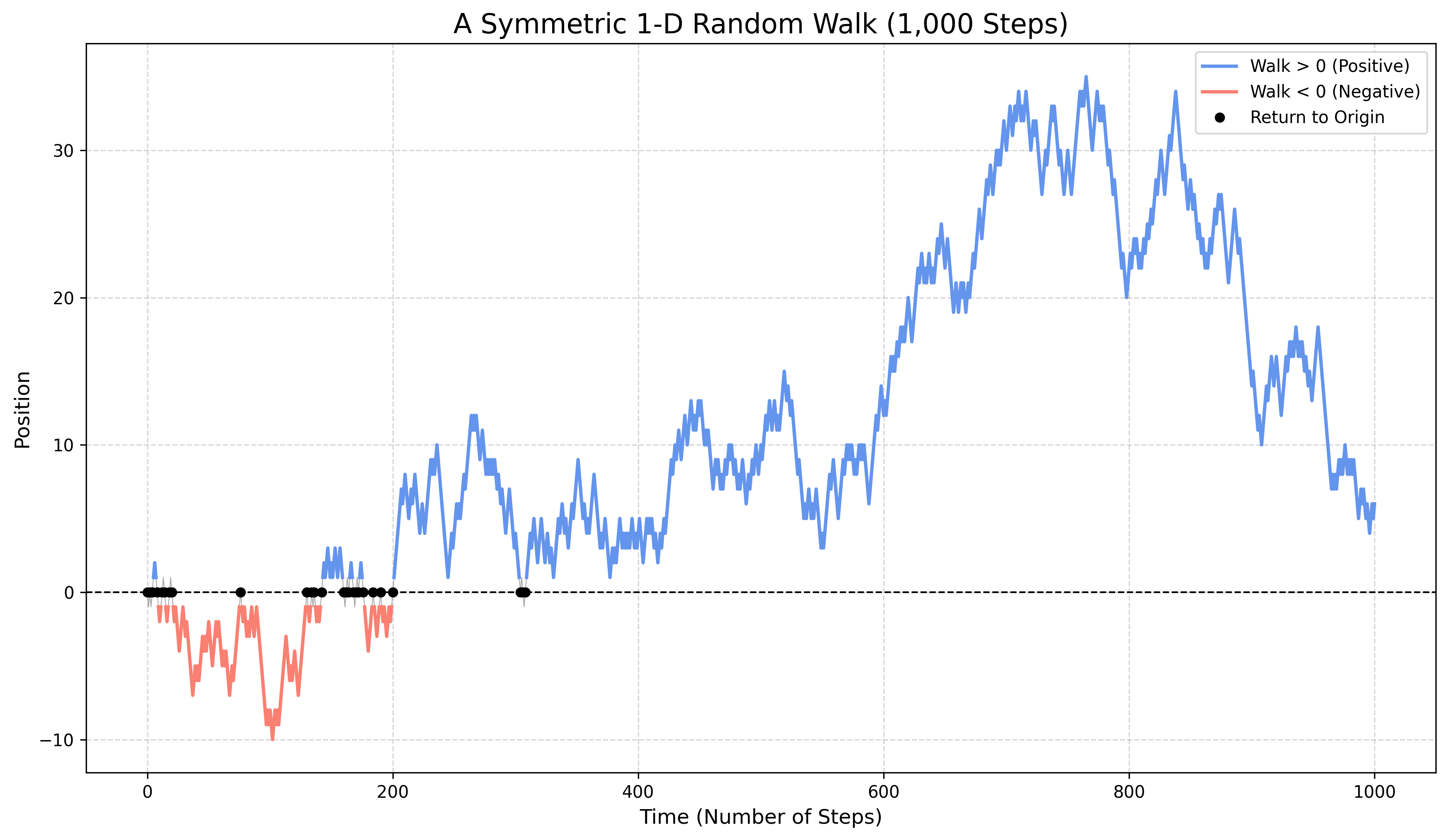
This note explores some features of a \(1\)-dimensional random walk. We consider a random walker who, each second, may take a step up with probability \(p\) or a step down with probability \(1-p\). For \(p=1/2\), the walker will get back to the origin with probability \(1\). One may then study the statistical properties of the random walk while the walker is away from \(0\). Some statements are proved with different methods in different sections.
This page contains interactive content, feel free to explore and modify it. For more involved modifications, you are encouraged to run and edit the interactive Jupyter Notebook instead. You can either:
- Run it on a computer with a Python/Jupyter-lab installation (requires
ipywidgets,numpy,matplotlib). - Run it using an online service. The official Jupyter website provides a free and open service. If you need more computing power, you can import the notebook in Google Colab (requires a Google account).
Definitions
We begin with a formal definition of the random walk.
Definition 1 (1-d Random Walk) Let \((X_i)_{i\ge 1}\) be a sequence of i.i.d. random variables with \[ \mathbb P(X_i = +1) = p \quad \text{and} \quad \mathbb P(X_i = -1) = 1-p \] for some \(p \in [0,1]\). The 1-dimensional random walk starting at the origin is the sequence of random variables \((S_n)_{n\ge 0}\) defined by \(S_0 := 0\) and \[ S_n := \sum_{i=1}^n X_i \quad \text{for } n \ge 1 \tag{1}\] The walk is called symmetric if \(p=1/2\) and asymmetric otherwise. We say the walker returns to the origin at time \(n\) if \(S_n=0\). The first return time to the origin is the random variable \[ \tau_0 := \inf \{ n \ge 1 \,:\, S_n = 0 \} \tag{2}\] where we set \(\inf \emptyset = \infty\).
We first determine for which values of \(p\) the walker is certain to return to the origin, namely \(\mathbb P(\tau_0 < \infty) = 1\). Such a walk is called recurrent. If \(\mathbb P(\tau_0 < \infty) < 1\), the walk is called transient.
Will the walker get back to the origin?
The behavior of the walk is dramatically different in the symmetric versus the asymmetric case.
The asymmetric case: escaping to infinity
If the walk is biased (\(p\ne 1/2\)), there is a net drift in one direction. The Strong Law of Large Numbers (SLLN) is sufficient to show that the walker almost surely moves away from the origin forever.
Proposition 1 If \(p \neq 1/2\), the 1-d random walk is transient. In fact, \(|S_n| \to \infty\) almost surely, which implies that the walker visits the origin only a finite number of times.
Proof (Proposition 1). The mean of a single step is \(m := \mathbb E[X_i] = 2p-1\). This \(m\neq 0\) iff \(p \neq 1/2\). By the Strong Law of Large Numbers, we have almost surely \[ \lim_{n\to\infty} \frac{S_n}{n} = m \] This implies that, if \(m\neq 0\), \(|S_n| \to \infty\) almost surely. It thus can only take the value \(0\) finitely many times. Therefore, the walk is transient.
Remark. We have just checked that the number of times the walker gets back to \(0\) is finite, with probability \(1\) if \(p\neq 1/2\). A proper way to do it is to think that for each \(p\in [0,1]\) we have a probability measure \(\mathbb P_p\) on the space of trajectories \(\mathbf X \colon \mathbb N\to \mathbb Z\). Then define a random variable \[ \mathcal N_0 \equiv \mathcal N_0(\mathbf X):= |\{ n\in \mathbb N \,:\: S_n=0\}| \in \mathbb N \cup \{+\infty\} \] This is the number of times the walker visits the origin. Proposition 1 can also be written \[ \mathbb P(\mathcal N_0 <\infty)=1 \qquad p\neq 1/2 \]
Exercise 1 Let \(p\neq 1/2\). Prove that the random variable \(\mathcal N_0\) follows a geometric distribution \(\mathbb P(\mathcal N_0=k)=(1-\theta)^{k-1}\theta\) for \(k \ge 1\) and some \(\theta = \mathbb P(\tau_0=\infty)\in (0,1)\).
Exercise 2 The geometric distribution of \(\mathcal N_0\) in Exercise 1 depends on the parameter \(\theta\), which in turn depends on \(p\), let’s denote it \(\theta_p\). (Recall \(p\neq 1/2\)).
- Prove that \(\theta_p=\theta_{1-p}\).
- Prove that, for \(p>1/2\), \(p\mapsto \theta_p\) is strictly increasing. (Hint: draw two random walks, corresponding to \(p>q>1/2\). If the first step is \(-1\), they both will get back to \(0\). If the first step is \(+1\), can you realize them simultaneously so that the one with parameter \(p\) is never smaller than the one with parameter \(q\)?).
The symmetric case: a certain return
When the walk is symmetric, there is no drift. One might guess the walker could still drift away by chance. However, it turns out that a return to the origin is almost sure. A powerful way to see this is to analyze the expected number of returns.
For \(\tau_0^{(0)} :=0\), define for \(n\ge 1\) \[ \tau_0^{(n)}\equiv \tau_0^{(n)}(\mathbf X):= \inf \{m > \tau_0^{(n-1)} \,:\: S_m=0\} \] so that \(\tau_0 \equiv \tau_0^{(1)}\), see Equation 2. \(\tau_0^{(n)}\) is the \(n\)-th time the walk touches the origin. We have the simple fact \[ \mathbb P(\tau_0^{(n)}<\infty)= \mathbb P(\tau_0<\infty)^n \] since indeed each time we visit \(0\), the process restarts anew. So the probability that we come back \(n\) times, is exactly the probability that we come back once, to the power \(n\). This gives us a powerful tool to prove that \(\mathbb P(\tau_0<\infty)=1\). Indeed \[ \begin{aligned} & \sum_{m=0}^\infty \mathbb P(S_m=0)= \mathbb E\left[ \sum_{m=0}^\infty1_{S_m=0} \right]= \mathbb E\left[\sum_{n=0}^\infty 1_{\tau_0^{(n)}<\infty} \right] \\ & = \sum_{n=0}^\infty \mathbb P( \tau_0<\infty)^n = \frac{1}{1- \mathbb P( \tau_0<\infty)} \end{aligned} \] That is (both sides may be \(+\infty\)) \[ \mathbb E[\mathcal N_0]=\sum_{m=0}^\infty \mathbb P(S_m=0) = \frac{1}{1- \mathbb P( \tau_0<\infty)} \tag{3}\]
Proposition 2 If \(p = 1/2\), the 1-d symmetric random walk is recurrent, i.e., \(\mathbb P(\tau_0 < \infty) = 1\).
It is worth recalling the Stirling’s bounds for the factorial \[ n^n e^{-n} \sqrt{2\pi n} e^{1/(12 n+1)} \le n! \le n^n e^{-n} \sqrt{2\pi n} e^{1/ (12 n)} \qquad n\ge 1 \tag{4}\]
Proof (Proposition 2). For the walker to be at the origin at time \(n\), it must have taken an equal number of steps up and down. This is only possible if \(n\) is even. Let \(n=2k\) for some \(k\ge 1\). The number of paths of length \(2k\) is \(2^{2k}\). The number of paths with exactly \(k\) steps up and \(k\) steps down is given by the binomial coefficient \(\binom{2k}{k}\). Thus, the probability of being at the origin at time \(2k\) is \[ \mathbb P(S_{2k}=0) = \binom{2k}{k} \left(\frac{1}{2}\right)^{2k} \] If we use Stirling’s approximation (Equation 4) for the factorials in the last formula, we get for \(k\ge 1\) \[ \mathbb P(S_{2k}=0) = \frac{1}{\sqrt{\pi k}} (1-\varepsilon_k), \qquad \frac{1}{8k+3}\le \varepsilon_k\le \frac{1}{8k} \tag{5}\] Since the series \(\sum_k \mathbb P(S_{2k}=0)\) diverges, we get the statement thanks to Equation 3.
Proof (Another proof of Proposition 2). Let \(p_x\) be the probability that a walker starting at point \(x\) will eventually hit \(0\). We want to show that \(p_x=1\) for all \(x \in \mathbb Z\). Clearyl \(p_0=1\). For \(x \neq 0\), by conditioning on the first step, we have: \[ p_x = \frac{1}{2} p_{x-1} + \frac{1}{2} p_{x+1}, \qquad x\in \mathbb Z \setminus \{0\} \] This equation implies that the points \((x-1, p_{x-1})\), \((x, p_x)\), and \((x+1, p_{x+1})\) are collinear. The only line that passes through \((0,1)\) and remains bounded with \(0\le p_x \le 1\) for all \(x\) is the constant line \(p_x=1\). Thus, the walk is recurrent.
Exercise 3 Use the same approach to prove that for \(p\neq 1/2\), \(1-\theta_p=\mathbb P(\tau_0<\infty)<1\). Express \(\theta_p\) using a series.
Remark 1. The recurrence is not a trivial consequence of the symmetry. If we were to perform a symmetric walk on \(\mathbb Z^3\) (indeed on any finitely generated group which is not virtually isomorphic to \(\mathbb Z\) or \(\mathbb Z^2\)), the walk would be transient despite the symmetry. Informally speaking, recurrence is a consequence of the symmetry and the fact that \(\mathbb Z\) is a small graph.
Excursions
The statistical properties of the so called excursions turn out to be quite interesting. We give a brief overview of the law of the return time here.
Definition 2 (Excursion) A path segment \((S_m, S_{m+1}, \ldots, S_{m+n})\) is an an excursion from 0 of length \(n\) if \(S_m=0\), \(S_{m+n}=0\), and \(S_{m+k} \neq 0\) for all \(k \in \{1, \ldots, n-1\}\). Once the walker touches \(0\) the process restarts anew, the statistical properties of all excursions are identical. We can therefore focus on the first excursion, whose duration is given by the first return time \(\tau_0\).
Our goal is to compute the probability distribution of the length of an excursion, i.e., \(\mathbb P(\tau_0 = n)\). Note that if \(S_n=0\), \(n\) must be even, so we only need to compute \(\mathbb P(\tau_0=2k)\) for \(k\ge 1\). If the walk is not symmetric, such a length has a non-zero probability of being infinite.
Exercise 4 For \(|s|<1\) define \[ v(x,s):= \mathbb E_x[s^{\tau_0}] = \sum_{k=0}^\infty \mathbb P_x(\tau_0=k)s^k \] where \(\mathbb E_x\) means expected value for the random walk starting in the point \(x\) (this is the same as starting at \(0\) and hitting the point \(-x\)).
- Prove that \(v(x,s)= v(1,s)^x\) for \(x\ge 1\), and \(v(x,s)=v(-1,s)^{-x}\) for \(x\le -1\). Hint: starting at \(x=2\), we first need to hit \(1\), then from \(1\) need to hit \(0\).
- Use the previous fact to compute \(v(x,s)\) for all \(x,s\) including \(x=0\). Check in particular \[ v(0,s)=1-\sqrt{1-4 p(1-p)s^2}, \qquad v(1,s)=v(0,s)/(2 s p), \qquad v(-1,s)=v(0,s)/(2s (1-p)) \]
- Deduce \(\theta_p=\mathbb P_0(\tau_0=\infty)= |1-2p|\), which in particular proves the results of the previous section.
- Use the Taylor formula \[ 1- \sqrt{1-4t}= \sum_{n=1}^\infty A_n t^n, \qquad A_n=\frac{(2n)!}{(2n-1)(n!)^2} \] to deduce that \[ \mathbb P_0(\tau_0=2k)=A_k p^k (1-p)^k \tag{6}\]
One may have a purely combinatorial proof of the same fact.
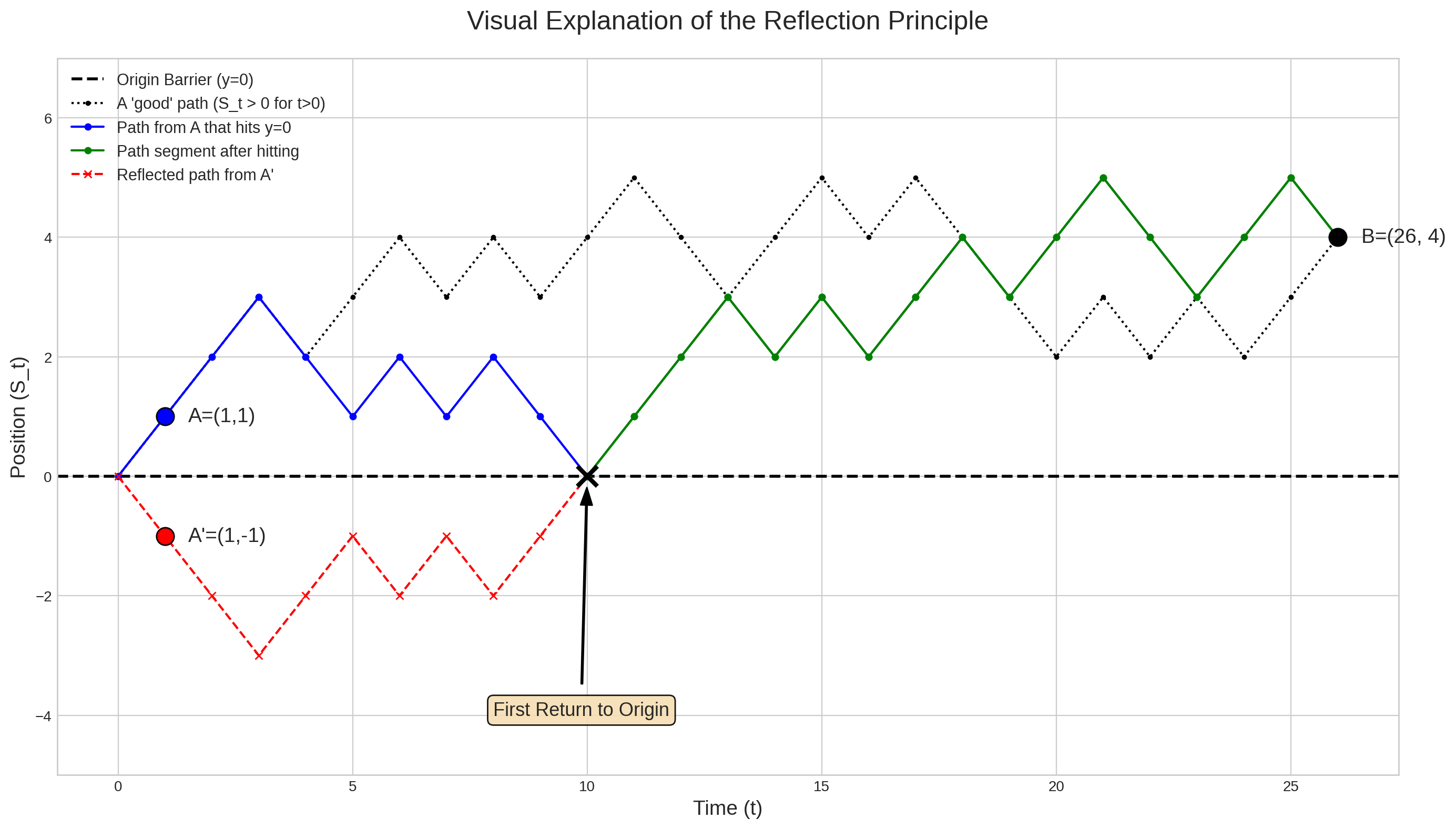
Lemma 1 (The Reflection Principle) Let \(S_n\) be a symmetric random walk. For any integers \(a>b>0\), the number of paths from the origin to the point \((n,b)\) that touch or cross the level \(a\) is equal to the number of paths from the origin to the point \((n, 2a-b)\).
Proof (Lemma 1). Let a path \((S_0, S_1, \ldots, S_n)\) start at \(S_0=0\) and end at \(S_n=b\). Suppose this path touches or crosses the level \(a\). Let \(k = \inf\{ j \ge 1 : S_j=a \}\) be the first time the path hits \(a\).
We can create a new, reflected path \((S'_0, \ldots, S'_n)\), providing an involutive bijection between paths crossing \(a\) and finishing at \(b\), and paths finishing at \(2a-b\). Define:
- For \(j \le k\), let \(S'_j = S_j\). The new path is identical to the old one up to the first time it hits \(a\).
- For \(j > k\), let \(S'_j = a - (S_j - a) = 2a - S_j\). We reflect the remainder of the path in the line \(y=a\).
The original path starts at \((0,0)\) and ends at \((n,b)\). The new path also starts at \((0,0)\) (since \(k\ge 1\)) and ends at \((n, S'_n) = (n, 2a - S_n) = (n, 2a-b)\).
Exercise 5 Use Lemma 1 to prove directly \(\mathbb P_0(\tau_0=2k)=A_k p^k (1-p)^k\) counting the paths starting and finishing at \(0\) for the first time after \(2k\) steps.
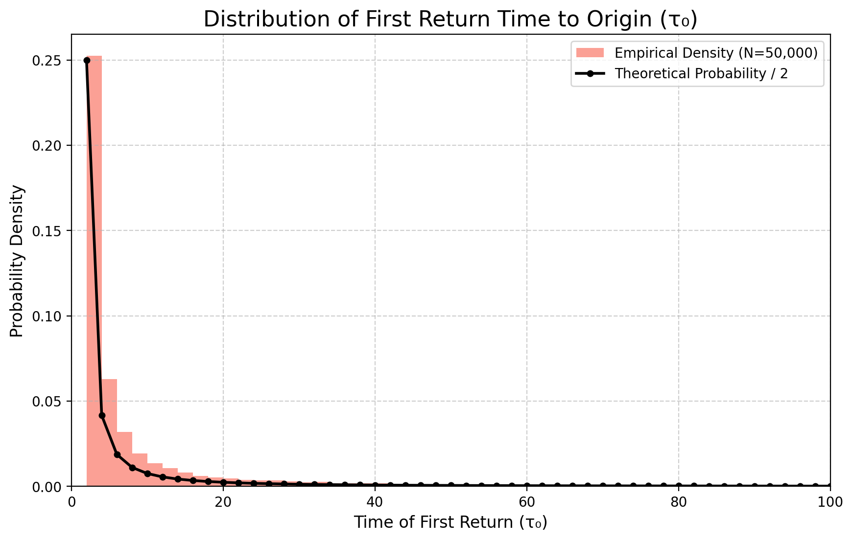
Remark. Using Stirling’s approximation on Equation 6, we find that for \(p=1/2\) \[ \mathbb P(\tau_0=2k) \approx \frac{1}{2\sqrt{\pi}} k^{-3/2} (1+o_k(1)) \] Thus \(\mathbb E[\tau_0]= \sum_k 2k \mathbb P(\tau_0=2k)=\infty\). This means that while a return is certain, \(\sum_k \mathbb P(\tau_0=2k)=1\), the expected time of the first return is infinite.
Exercise 6 (Paths in the positive half-plane) For a symmetric walk, find the number of paths from \((0,0)\) to \((n,y)\) (with \(y>0\)) that remain strictly positive for all times \(k \in \{1, \ldots, n\}\).
The path must start with a step to \((1,1)\). It must then go from \((1,1)\) to \((n,y)\) in \(n-1\) steps without hitting the level \(y=0\). The total number of paths from \((1,1)\) to \((n,y)\) is \(N((1,1)\to(n,y))\). By the reflection principle (Lemma 1 with \(a=1\)), the number of paths that touch level \(0\) is the number of paths from \((1,-1)\) to \((n,y)\), i.e., \(N((1,-1)\to(n,y))\). The desired number of paths is therefore: \[ N_{>0} = N((1,1)\to(n,y)) - N((1,-1)\to(n,y)) \] Using the formula \(N((s,a)\to(t,b)) = \binom{t-s}{(b-a+t-s)/2}\), this becomes: \[ N_{>0} = \binom{n-1}{(y-1+n-1)/2} - \binom{n-1}{(y-(-1)+n-1)/2} = \frac{y}{n} \binom{n}{(n+y)/2} = \frac{y}{n} N((0,0)\to(n,y)) \]
Exercise 7 (Maximum at the endpoint) Find the number of paths from \((0,0)\) to \((n,y)\) such that \(S_k < y\) for all \(k \in \{0, \ldots, n-1\}\).
This problem is symmetric to the previous one. Consider the time-reversed path from \((n,y)\) to \((0,0)\). This is a path of length \(n\) from \((0,0)\) to \((n,-y)\). The condition \(S_k < y\) on the original path is equivalent to the new path \(S'_k > -y\) for \(k \in \{1, \ldots, n\}\). By flipping the sign, this is the same as the number of paths from \((0,0)\) to \((n,y)\) that stay strictly positive. The answer is therefore the same as in Exercise 6: \(\frac{y}{n} N((0,0)\to(n,y))\).
Exercise 8 (Dyck paths) Find the number of symmetric random walk paths from \((0,0)\) to \((2n,0)\) that remain non-negative, i.e., \(S_k \ge 0\) for all \(k \in \{0, \ldots, 2n\}\).
This is a classic problem for Dyck paths. The answer is the \(n\)-th Catalan number, \(C_n\). \[ C_n = \frac{1}{n+1} \binom{2n}{n} \] This can be derived using the reflection principle. The total number of paths from \((0,0)\) to \((2n,0)\) is \(\binom{2n}{n}\). The number of “bad” paths (those that drop below the axis) is the number of paths that touch or cross the line \(y=-1\). By the reflection principle, this is equal to the number of paths from \((0,0)\) to \((2n,-2)\), which is \(\binom{2n}{n-1}\). The number of good paths is the difference: \[ \binom{2n}{n} - \binom{2n}{n-1} = \frac{1}{n+1}\binom{2n}{n} \]
Exercise 9 (Bridges) Find the number of symmetric random walk paths from \((0,0)\) to \((2n,0)\) with strictly positive intermediate vertices, i.e., \(S_k > 0\) for \(k \in \{1, \ldots, 2n-1\}\).
Such a path must start with a step to \((1,1)\) and end with a step from \((2n-1,1)\). The path segment from \((1,1)\) to \((2n-1,1)\) has length \(2n-2\) and must not drop below level \(y=1\). This is equivalent to a non-negative path of length \(2n-2\) from \((0,0)\) to \((0,0)\). From Exercise 8 (with \(n\) replaced by \(n-1\)), this number is the \((n-1)\)-th Catalan number: \[ C_{n-1} = \frac{1}{n} \binom{2n-2}{n-1} \]
The arcsin law
A surprising result concerns the time a symmetric random walk spends on one side of the axis. It turns out that the most likely scenarios are for the walker to spend almost all its time on the positive side, or almost all its time on the negative side. This is quantified by the arcsine law. Hereafter we assume \(p=1/2\).
To state the result precisely, we need a suitable definition for the time spent on the positive side. Let \(\pi_{2n}\) be the number of segments of the path \((S_0, S_1, \ldots, S_{2n})\) that lie on or above the horizontal axis. That is, \[ \pi_{2n} := |\{k \in \{1, \ldots, 2n\} : S_{k-1} \ge 0 \text{ and } S_k \ge 0 \}| \] Note that since \(S_k\) can only change by \(\pm 1\) at each step, a path cannot cross from \(S_{k-1} > 0\) to \(S_k < 0\) (or vice-versa) in a single step without passing through \(0\). This implies that \(\pi_{2n}\) must be an even integer.
We also define \[ L_{2n} = \max\{m \le 2n : S_m=0\} \] as the time of the last visit to the origin up to time \(2n\).
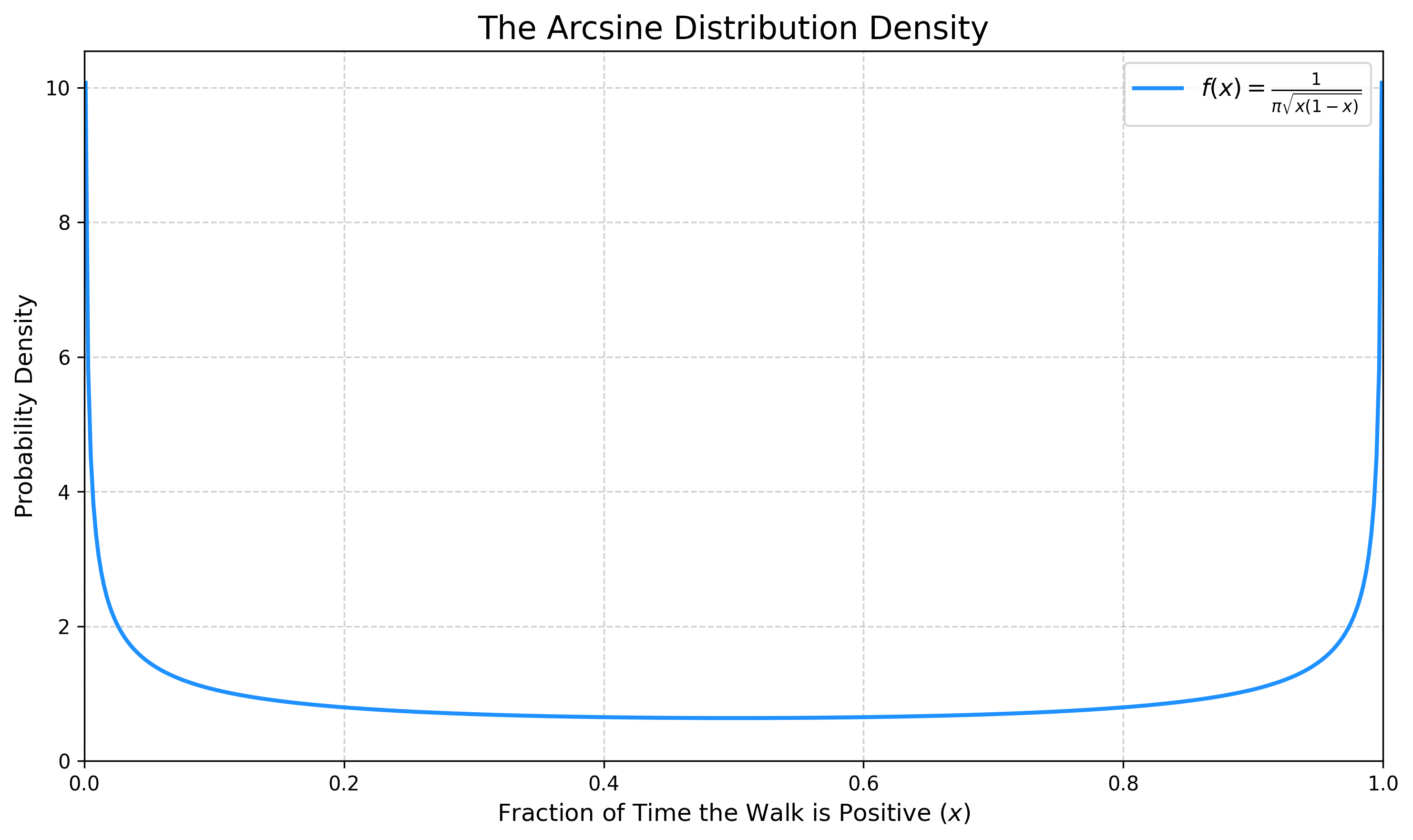
Theorem 1 (Lévy’s Arcsine Law) Let \((S_n)_{n\ge 0}\) be a symmetric 1-d random walk and \(\pi_{2n}\) the number of segments on or above the axis, as defined above. The fraction of time \(\pi_{2n}/(2n)\) converges in distribution to the arcsine distribution on \([0,1]\): \[ \lim_{n\to\infty} \mathbb P\left( \frac{\pi_{2n}}{2n} \le x \right) = \frac{2}{\pi} \arcsin(\sqrt{x}) \] for any \(x\in[0,1]\).
Moreover \(L_{2n}\) has the same distribution as \(\pi_{2n}\) and thus the same result holds for \(L_{2n}\)
The density of the arcsine distribution, \(\varrho(x) = (\pi\sqrt{x(1-x)})^{-1}\), is U-shaped, confirming that the walker most likely spends their time either on the positive or negative side of the axis.
The core idea of the proof is to find an exact expression for \(\mathbb P(\pi_{2n}=2k)\) for finite \(n\), and then use Stirling’s approximation to find the limit. For clarity we denote \(N\big((s,a)\to (t,b))\) the number of paths going from the point \(a\) at time (number of steps) \(s\) to the point \(b\) at time \(t\). This is \[ N\big((s,a)\to (t,b))= \binom{t-s}{(b-a +t-s)/2} \] meaning \(0\) if \((b-a +t-s)\) is odd.
Lemma 2 Then \[ \mathbb P(L_{2n}=2k) = u_{2k} u_{2(n-k)} \tag{7}\] where \(u_{2m}\) is the probability of being at \(0\) after \(2m\) steps, \(u_{2m}=\binom{2m}{m} 4^{-m}\).
Proof (Lemma 2). Let’s start from the case \(k=n\), that is let’s show \(\mathbb P(\tau_0 > 2n) = u_{2n}\). A path does not return to \(0\) iff it stays strictly on the positive side or strictly on the negative side. By symmetry, these two probabilities are equal. Let’s calculate the probability of staying strictly positive, \(P(S_1 > 0, \ldots, S_{2n} > 0)\), that is \(S_1=1\) and the subsequent \(2n-1\) steps starting from \(1\) never hitting \(0\).
The number of such paths can be found using the reflection principle (Lemma 1). The total number of paths from \((1,1)\) that stay strictly above \(0\) for \(2n-1\) steps is given by the result of the following telescopic sum over all possible final positions \(2r > 0\):
\[ \begin{aligned} & \sum_{r=1}^\infty \left[ N\big((1,1)\to(2n,2r)\big) - N\big((1,-1)\to(2n,2r)\big) \right] \\ & = \sum_{r=1}^\infty \left[ N\big((0,0)\to(2n-1,2r-1)\big) - N \big((0,0)\to(2n-1,2r+1)\big) \right] = \\ & N \big((0,0)\to(2n-1,1)\big) =\binom{2n-1}{n} \end{aligned} \]
For the symmetric walk, all paths have the same probability. So we can find the probability of not returning to the origin: \[ \mathbb P(\tau_0 > 2n) =2 \mathbb P(S_1=1, S_2 \ge 1,\ldots S_{2n}\ge 1) = 2 \binom{2n-1}{n} 2^{-2n} = u_{2n} \]
Now let’s consider the generic case \(k\le n\). The event \(\{L_{2n}=2k\}\) means that the walk is at the origin at time \(2k\), and does not return to the origin between times \(2k+1\) and \(2n\). We can write this as: \[ \mathbb P(L_{2n}=2k) = \mathbb P(S_{2k}=0 \text{ and } S_j \neq 0 \text{ for } 2k < j \le 2n) \] But the event \(\{S_{2k}=0\}\) is independent of the subsequent path: \[ \mathbb P(L_{2n}=2k) = \mathbb P(S_{2k}=0) \, \mathbb P(\tau'_0 > 2n-2k) \] where \(\tau'_0\) is the first return time for a new walk starting at \(0\) at time \(2k\). Using the result for \(k=n\) this becomes: \[ \mathbb P(L_{2n}=2k) = u_{2k} u_{2(n-k)} \]
Exercise 10 Define \(\alpha_{2k,2n}=\mathbb P(\pi_{2n}=2k)\). We want to prove that \(\alpha_{2k,2n}=u_{2k} u_{2(n-k)}\). Let \(f_{2m}=\mathbb P(\tau_0=2m)\).
- Prove that \(\alpha_{2k,2}= u_{2k} u_{2-2k}\) for \(k=0,1\).
- Prove that \(\alpha_{2n,2n}=u_{2n}\).
- Proceed by induction over \(n\) to check that, for \(k=1,\ldots,n-1\) \[ \alpha_{2k,2n}=\tfrac 12 u_{2n-2k}\sum_{m=1}^k f_{2m} u_{2k-2m} + \tfrac 12 u_{2k}\sum_{m=1}^{n-k} f_{2m} u_{2n -2k-2m} \]
- Conditioning on the time of first return, check that \(u_{2k}=\sum_{m=1}^k f_{2m} u_{2(k-m)}\).
- Use points c. and d. to conclude.
From Lemma 2 and Exercise 10, we get: \[ \mathbb P(\pi_{2n}=2k) = \mathbb P(L_{2n}=2k)= u_{2k} u_{2(n-k)} = \binom{2k}{k} \binom{2(n-k)}{n-k} 4^{-n} \tag{8}\]
We can now prove the theorem.
Proof (Theorem 1). We are interested in the cumulative distribution of the fraction of time \(\frac{\pi_{2n}}{2n}\). Let \(x \in (0,1)\), then \[ \mathbb P\left( \frac{\pi_{2n}}{2n} \le x \right) = \sum_{j=0}^{\lfloor nx \rfloor} \mathbb P(\pi_{2n}=2j) = \int_0^{\lfloor nx \rfloor/n} \varrho_n(y) dy \tag{9}\] where \[ \varrho_n(y):= n \mathbb P(\pi_{2n}=2j) \qquad \text{for $j/n \le y \le (j+1)/n $} \] By Equation 5 and Equation 8 \[ n \mathbb P(\pi_{2n}=2j)=n u_{2j} u_{2(n-j)}= \frac{1}{\sqrt{\pi j/n}} \frac{1}{\sqrt{\pi(1-j/n)}} (1-\varepsilon_j) (1-\varepsilon_{n-j}) \] and we immediately see that \(\varrho_{n}(x)\to \varrho(x)= (\pi\sqrt{x(1-x)})^{-1}\) uniformly on compact sets of \((0,1)\). Thus, passing to the limit \(n\to \infty\) in Equation 9 we get the theorem.
The equality in distribution of \(\pi_{2n}\) and \(L_{2n}\) is in Equation 8.
Multi-dimensional Random Walk
A natural generalization is the random walk on the \(l\)-dimensional integer lattice \(\mathbb{Z}^l\). The walker starts at a point \(\mathbf{x} \in \mathbb{Z}^l\), \(\mathbf{S}_0 = \mathbf{x} \in \mathbb{Z}^l\). At each step, it moves to one of the \(2l\) neighboring points with equal probability \(1/(2l)\). That is, \(\mathbf{S}_n = x + \sum_{i=1}^n \mathbf{X}_i\), where \(\mathbf{X}_i\) are independent random vectors taking values \(\pm \mathbf{e}_j\) (where \(\mathbf{e}_j\) are the standard basis vectors) with probability \(1/(2l)\).
As in the one-dimensional case, we can ask whether the walk is recurrent (returns to the origin with probability \(1\)) or transient. The answer, it turns out, depends on the dimension \(l\).
Characteristic function and transition probabilities
To analyze the multi-dimensional case, the characteristic function is a convenient tool. Let \(\mathbb{P}_{\mathbf{x}}(\mathbf{S}_n = \mathbf{y})\) be the probability that a walk starting at \(\mathbf{x}\) is at point \(\mathbf{y}\) after \(n\) steps. The characteristic function of the random vector \(\mathbf{S}_n\) (conditional on starting at \(\mathbf{x}\)) is defined as: \[ F(\mathbf{\theta}, n, \mathbf{x}) = \mathbb{E}_{\mathbf{x}}[e^{i \mathbf{\theta} \cdot \mathbf{S}_n}] = \sum_{\mathbf{y} \in \mathbb{Z}^l} \mathbb{P}_{\mathbf{x}}(\mathbf{S}_n = \mathbf{y}) e^{i \mathbf{\theta} \cdot \mathbf{y}} \] where \(\mathbf{\theta} = (\theta_1, \ldots, \theta_l) \in \mathbb{T}^l \simeq (-\pi, \pi]^l\). Due to the independence of steps, we have: \[ F(\mathbf{\theta}, n, \mathbf{x}) = e^{i \mathbf{\theta} \cdot \mathbf{x}} \left( \mathbb{E}[e^{i \mathbf{\theta} \cdot \mathbf{X}_1}] \right)^n \] The expectation for a single step is: \[ \mathbb{E}[e^{i \mathbf{\theta} \cdot \mathbf{X}_1}] = \sum_{j=1}^l \frac{1}{2l} (e^{i\theta_j} + e^{-i\theta_j}) = \frac{1}{l} \sum_{j=1}^l \cos(\theta_j) =: \Phi(\mathbf{\theta}) \] Thus, \(F(\mathbf{\theta}, n, \mathbf{x}) = e^{i \mathbf{\theta} \cdot \mathbf{x}} [\Phi(\mathbf{\theta})]^n\). The transition probabilities can be recovered via the inverse Fourier transform: \[ \mathbb{P}_{\mathbf{x}}(\mathbf{S}_n = \mathbf{y}) = \frac{1}{(2\pi)^l} \int_{(-\pi, \pi]^l} F(\mathbf{\theta}, n, \mathbf{x}) e^{-i \mathbf{\theta} \cdot \mathbf{y}} d\mathbf{\theta} = \frac{1}{(2\pi)^l} \int_{(-\pi, \pi]^l} e^{i \mathbf{\theta} \cdot (\mathbf{x}-\mathbf{y})} [\Phi(\mathbf{\theta})]^n d\mathbf{\theta} \tag{10}\]
Pólya’s Criterion: Recurrence and Transience
We have seen in Exercise 1 (which easily holds in any dimension), that if the walk is transient, then the number of returns to \(0\) is a geometric random variable, thus it has finite expectation. Therefore the walk is recurrent iff the expected number of returns to the origin is infinite. Let’s denote this expectation by \(g(\mathbf{0}, \mathbf{0}) = \sum_{n=0}^\infty \mathbb{P}_{\mathbf{0}}(\mathbf{S}_n = \mathbf{0})\). Using Equation 10, since \(|\Phi(\mathbf{\theta})| < 1\) but in two points (\(\theta_1=\ldots=\theta_l=0\) and \(\theta_1=\ldots=\theta_l=\pi\)):
\[ g(\mathbf{0}, \mathbf{0}) = \sum_{n=0}^\infty \frac{1}{(2\pi)^l} \int_{(-\pi, \pi]^l} [\Phi(\mathbf{\theta})]^n d\mathbf{\theta} = \frac{1}{(2\pi)^l} \int_{(-\pi, \pi]^l} \sum_{n=0}^\infty [\Phi(\mathbf{\theta})]^n d\mathbf{\theta} = \frac{1}{(2\pi)^l} \int_{(-\pi, \pi]^l} \frac{1}{1 - \Phi(\mathbf{\theta})} d\mathbf{\theta} \]
The walk is recurrent if this integral diverges, and transient if it converges. The convergence is determined by the behavior of the integrand near the points where the denominator is zero, i.e., \(\mathbf{\theta} \approx \mathbf{0}\). Near the origin, \(\cos(\theta_j) \approx 1 - \theta_j^2/2\), so: \[ 1 - \Phi(\mathbf{\theta}) = 1 - \frac{1}{l} \sum_{j=1}^l \cos(\theta_j) \approx 1 - \frac{1}{l} \sum_{j=1}^l (1 - \theta_j^2/2) = \frac{1}{2l} \sum_{j=1}^l \theta_j^2 = \frac{\|\mathbf{\theta}\|^2}{2l} \] Thus, the convergence of the integral depends on the convergence of \(\int \frac{d\mathbf{\theta}}{\|\mathbf{\theta}\|^2}\) near the origin. In polar coordinates, \(d\mathbf{\theta} \sim r^{l-1}dr\), so the integral behaves like \(\int_0 \frac{r^{l-1}}{r^2} dr = \int_0 r^{l-3} dr\).
- For \(l=1\), the integral \(\int r^{-2}dr\) diverges. The walk is recurrent.
- For \(l=2\), the integral \(\int r^{-1}dr\) diverges. The walk is recurrent.
- For \(l \ge 3\), the exponent \(l-3 \ge 0 > -1\), so the integral converges. The walk is transient.
This result is known as Pólya’s Theorem: the symmetric random walk on \(\mathbb{Z}^l\) is recurrent for \(l=1,2\) and transient for \(l \ge 3\). This is a special case of the result stated in Remark 1.
Simulating the walk
We can easily check numerically the various statements, since the convergence takes place quite quickly.
First return to \(0\)
We first computed explicitly the law of the first return to \(0\). Its expected value is infinite, so one has to be careful in the simulation, and cut off the simulations at a given number of steps. This introduces a bias that we report, but do not compensate here since it is a negligible effect at this precision.
Arcsin law
Then we simulate via Monte Carlo the amount of time the random walk stays positive.
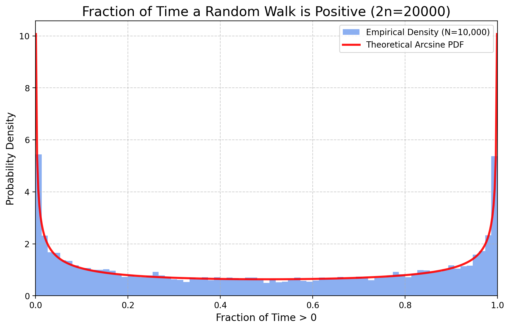
Roughly speaking, these distributions are universal, meaning that they represent the scaling limit of several different random dynamics. For instance, we can change the law of the \(X_i\) to any centered distribution with finite variance (say \(1\)), to converge to the same law.
In this plot a continuous uniform distribution is used.

You can try to check the universality of the arcsin distribution. You can check what happens for different distributions. If the distributions are centered but not symmetric (e.g. a centered exponential \(X-\mathbb E[X]\) with \(X\) exponential), what do
#| '!! shinylive warning !!': |
#|   shinylive does not work in self-contained HTML documents.
#|   Please set `embed-resources: false` in your metadata.
#| standalone: true
#| components: [editor, viewer]
#| viewerHeight: 1080
#| editorHeight: 240
#| layout: vertical

# ========= 1. IMPORTS & CONFIGURATION =========
from shiny import App, render, ui, reactive, req
import numpy as np
import matplotlib.pyplot as plt

# Configuration dictionary for UI inputs
ARCSIN_CONFIG = {
    'n_slider': {
        'min': 10, 'max': 2000, 'value': 200, 'step': 2,
    },
    'N_samples_slider': {
        'min': 100, 'max': 10000, 'value': 5000, 'step': 100,
    },
    'distribution': {
        'choices': ['Symmetric {-1, +1}', 'Standard Normal N(0,1)', 'Uniform [-1, 1]', 'Centered Exponential'],
        'selected': 'Symmetric {-1, +1}',
    },
    'filename': {'value': 'arcsin_simulation.png'},
}

# ========= 2. UI DEFINITION =========
app_ui = ui.page_sidebar(
    ui.sidebar(
        ui.h3("Arcsine Law Simulation"),
        ui.p("This simulation shows the distribution of the fraction of time a 1-D random walk spends on the positive side."),
        ui.hr(),
        ui.input_slider("n", "Number of Steps (2n):", **ARCSIN_CONFIG['n_slider']),
        ui.input_slider("N_samples", "Number of Walks (N):", **ARCSIN_CONFIG['N_samples_slider']),
        ui.input_select("distribution", "Step Distribution:", **ARCSIN_CONFIG['distribution']),
        ui.hr(),
        ui.input_action_button("run_button", "Run Simulation", class_="btn-success w-100"),
        ui.hr(),
        ui.h4("Saving Options"),
        ui.input_checkbox("save_plot", "Save Plot", value=False),
        ui.panel_conditional(
            "input.save_plot",
            ui.input_text("filename", "Filename:", **ARCSIN_CONFIG['filename']),
        ),
        title="Controls",
    ),
    ui.output_plot("arcsin_plot", height="700px"),
    title="Arcsine Law for Random Walks",
)

# ========= 3. SERVER LOGIC =========
def server(input, output, session):
    figure_to_display = reactive.Value(None)

    # --- Helper Functions ---
    def generate_steps(dist_name, size):
        """Generates random steps based on the selected distribution."""
        if dist_name == 'Symmetric {-1, +1}':
            return np.random.choice([-1, 1], size=size)
        if dist_name == 'Standard Normal N(0,1)':
            return np.random.randn(*size)
        if dist_name == 'Uniform [-1, 1]':
            return np.random.uniform(-1, 1, size=size)
        if dist_name == 'Centered Exponential':
            # Asymmetric distribution with mean 0
            return np.random.standard_exponential(size=size) - 1
        raise ValueError(f"Unknown distribution: {dist_name}")

    def get_arcsin_pdf(x):
        """Calculates the PDF of the Arcsine distribution."""
        return 1 / (np.pi * np.sqrt(x * (1 - x)))

    @reactive.Effect
    @reactive.event(input.run_button, ignore_init=True)
    def _():
        """Runs the simulation when the action button is clicked."""
        n = input.n()
        N = input.N_samples()
        dist_name = input.distribution()

        try:
            # --- Perform Simulation ---
            steps = generate_steps(dist_name, size=(N, n))
            walks = np.cumsum(steps, axis=1)
            time_positive = np.sum(walks > 0, axis=1)
            fractions = time_positive / n

            # --- Create Plot ---
            fig, ax = plt.subplots(figsize=(10, 6))
            num_bins = min(80, max(20, N // 100))
            ax.hist(fractions, bins=num_bins, density=True, alpha=0.75,
                    label=f'Empirical Density (N={N:,})')

            # --- Plot Theoretical PDF (only if applicable) ---
            symmetric_dists = ['Symmetric {-1, +1}', 'Standard Normal N(0,1)', 'Uniform [-1, 1]']
            if dist_name in symmetric_dists:
                x_axis = np.linspace(1e-4, 1 - 1e-4, 500)
                ax.plot(x_axis, get_arcsin_pdf(x_axis), 'r-', lw=2.5, alpha=0.9,
                        label='Theoretical Arcsine PDF')

            # --- Customize Plot ---
            ax.set_title(f"Fraction of Time Positive (Steps ~ {dist_name}, 2n={n})")
            ax.set_xlabel("Fraction of Time > 0")
            ax.set_ylabel("Probability Density")
            ax.set_xlim(0, 1)
            ax.set_ylim(bottom=0)
            ax.legend()
            ax.grid(True, linestyle='--', alpha=0.6)

            # --- Handle Saving ---
            if input.save_plot():
                req(input.filename(), cancel_output=True)
                fig.savefig(input.filename(), dpi=400, bbox_inches='tight')

            figure_to_display.set(fig)
            plt.close(fig)

        except Exception as e:
            fig, ax = plt.subplots()
            ax.text(0.5, 0.5, f"An error occurred: {e}", ha='center', va='center', wrap=True)
            figure_to_display.set(fig)
            plt.close(fig)

    @output
    @render.plot
    def arcsin_plot():
        """Renders the plot from the reactive value."""
        fig = figure_to_display.get()
        req(fig)
        return fig

# ========= 4. APP INSTANTIATION =========
app = App(app_ui, server)
Recurrence and transience in higher dimension
If we run a 3-d random walk, say \(X\), and take its projection \(Y\) on a horizontal plane, the projected walk will not move when \(X\) moves vertically. But if we skip this time (which will not change the property of coming back to \(0\) or not), \(Y\) just performs a 2-d random walk. It is clear that \(Y\) will intersect its own path (come back where it was) much more often than \(X\). Indeed, each time \(X\) comes back to \(0\), \(Y\) will also do it, while the opposite is not true (when \(Y\) is at the origin, \(X\) may be at some point \((0,0,z)\)). This is even more true if we project on just one coordinate axis. In other words, it is clear that the higher the dimension, the more transient the walk is (for symmetric random walks). This informal argument can be easily turned into a rigorous proof. This video shows the phenomenon described.